The Beta Distribution

We build an intuitive understanding of the Beta distribution and its utility as a prior distribution for many other probability distributions.

The beta distribution models a distribution of probabilities. If we don’t know the probability of the outcome of an event, we can use the beta distribution to model the distribution of probabilities given the prior information.

For example, assume you have a webshop. For every visitor to your site, you are ultimately interested in whether the customer buys or leaves without buying. It is a binary outcome which we can model using a Bernoulli trial.

Let’s say you have 20 customers. 10 of them buy and 10 leave without buying. The average probability of making a purchase or conversion rate is now 50% (0.5). But 20 people isn’t a very reliable sample size. Your real probability of converting customers could be lower or higher. The beta distribution accounts for this problem by giving you a distribution of possible conversion rates and their associated probabilities of reflecting the real conversion rate in light of the empirical evidence.

Here is the beta distribution for 20 customers with 10 sales.

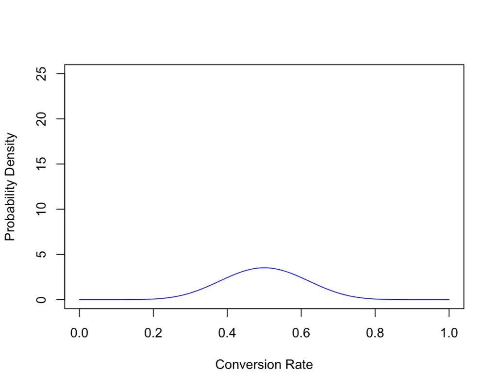
As you see, the chance that the real conversion rate falls somewhere in the area around 0.5 has the highest associated probability, but the real conversion rate could lie anywhere. However, the probability that it lies below 0.2 or above 0.8 is vanishingly small.

Now you collect a bit more data. After 200 customers, it turns out 80 have bought something while 120 have not.

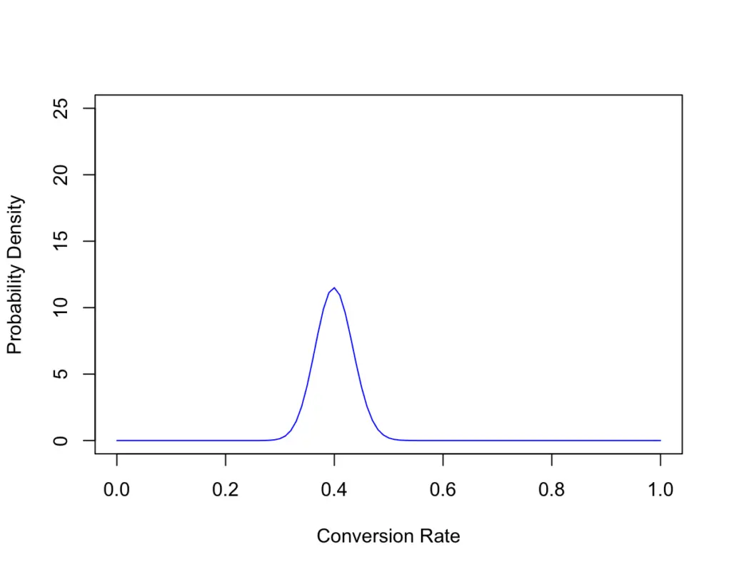
As a reflection of our new data, our most probable conversion rate now falls into the area of 0.4. But something else has happened. The probability of the area around 0.4 reflecting the actual conversion rate is much higher, while the tails are not as wide anymore. Since we have more empirical evidence, we were able to increase our confidence that the real conversion rate is roughly 0.4, while the range around 0.8 has become much more improbable.

Now you perform some modifications on your site to improve your sales.

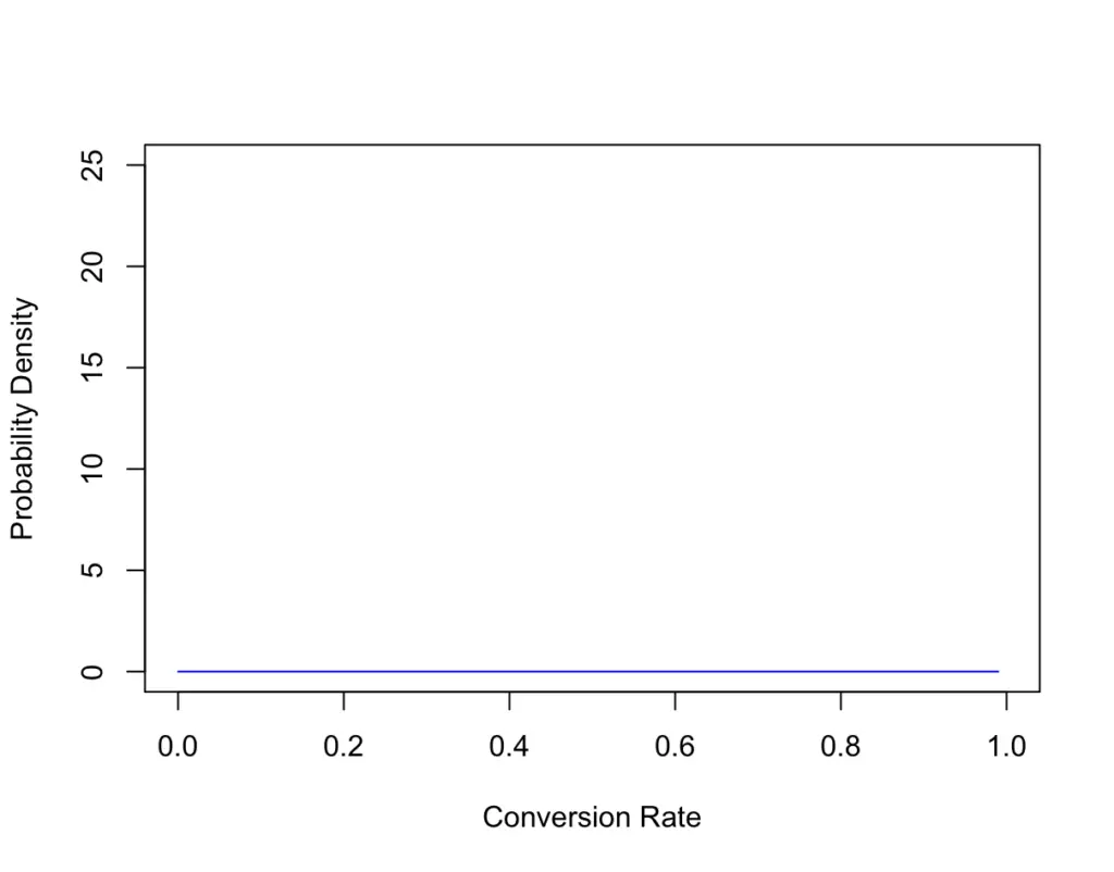
After your modifications, you don’t know the probability that a new customer will buy. Suppose the first customer buys. Your conversion rate is 100%. But of course, it would be unreasonable to infer from one sale that all future customers will make a purchase. So the probability that the real conversion rate is 100% is effectively zero. The beta distribution accounts for this lack of evidence.

Instead, you could use your previously collected data (80 sales for 200 visitors) as a prior and then you gradually update your distribution as you collect more data.

Let’s say you wait for another 100 customers and 80 of them buy. Now you have a total of 160 sales out of 300 visitors. Compared to your old data, this looks like a big improvement.

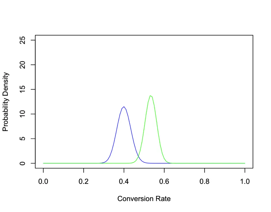
In the light of the collected data, we can be pretty confident that the actual conversion rate has improved after our changes. We cannot be certain though as indicated by the overlap of the blue and the green curves.

To calculate the exact probabilities, we have to take the integral over the area under the curve. We’ve done enough to build intuition, so let’s dive into the math next.

Beta Distribution Formula

As we said in the beginning, the beta distribution is a probability distribution over probabilities. It is often used for modeling the prior probability of binary events that are themselves Bernoulli distributed.

Recall that a Bernoulli trial is basically a product of factors of the following form.

P(X=x)=p^x
 (1−p) ^
{1−x}

In the real world, we probably don’t know the real value of p. In fact, p itself follows a probability distribution that we want to incorporate into our calculation. This is known as the prior.

We want to choose a prior proportional to the powers of p and (1-p) because then the posterior and the prior have the same functional form. This is a property known as conjugacy.

The beta distribution has the same functional form and is, therefore, an appropriate prior distribution to the Bernoulli distribution.

Using the Beta probability density function, we can model the prior probability of p using the parameters alpha and beta

Beta(p|\alpha,\beta) = \frac{\Gamma(\alpha + \beta)}{\Gamma(\alpha)\Gamma(\beta)} p^{\alpha-1} (1-p)^{\beta-1}

where Γ is the Gamma distribution.

The expression involving the gamma distribution normalizes the beta distribution to the interval [0,1].

Beta(\alpha, \beta) = \frac{\Gamma(\alpha)\Gamma(\beta)}{\Gamma(\alpha + \beta)}

Accordingly, we can express the Beta PDF as follows.

\frac{p^{\alpha-1}(1-p)^{\beta-1}}{Beta(\alpha, \beta) }

The expected value and variance are relatively straightforward.

E(p) = \frac{\alpha}{\alpha + \beta} \;\;\;

Var(p) = \frac{\alpha \beta}{(\alpha + \beta)^2(\alpha + \beta + 1)}

This post is part of a series on statistics for machine learning and data science. To read other posts in this series, go to the index.