Central Limit Theorem

In this post, we build an intuitive understanding of the central limit theorem by looking at some examples. Then, we introducing the formal definition of the CLT.

What is the Central Limit Theorem

The central limit theorem states that under most conditions, the sum of large numbers of random variables is normally distributed. This holds even if the random variables themselves are not normally distributed.

The central limit theorem is one of the most important ideas in statistics. It also explains why the normal distribution is so dominant.

Before diving into the mathematical explanation, let’s just build some intuition using the example of dice throws, which can be modeled using a binomial distribution.

Central Limit Theorem Example

Let’s say we roll one fair 6-sided dice 1000 times. We consider the outcome of each roll to be one sample. The distribution of results looks approximately like this.

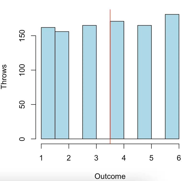
This looks very much like the uniform distribution which makes sense because each outcome is equally probable. Our expected value as indicated by the red line is 3.5. Of course, since we throw one dice, we will never get exactly the expected value.

Let’s roll a dice twice and take the average of both and repeat that process a thousand times. The outcome of both dice throws X1, X2 constitutes one sample X.

X = \{X_1,X_2\}

Then we calculate the sample mean.

\bar X = \frac{X_1,X_2}{2}

Plotting the sample means of our looks like this. This time I’ve also plotted the green line to indicate the sample mean. The expected value, again, is 3.5.

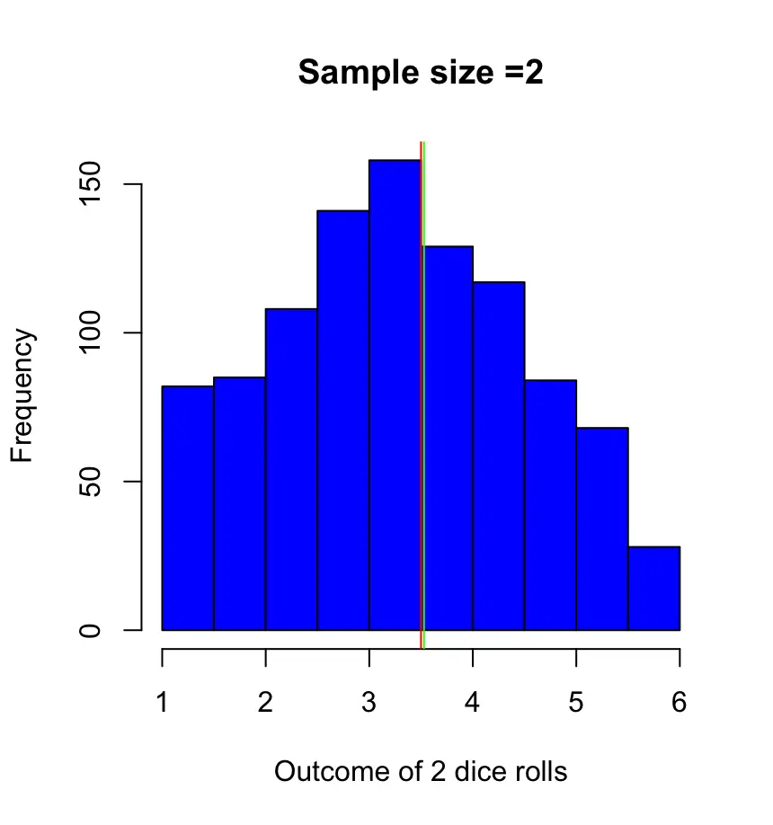
As you see, the means of most of our samples are close to the expected value. But, if you throw two dice a thousand times, you can reasonably expect to get twice 1 or twice 6 at least a couple of times. Then your average will be higher.

Let’s repeat the experiment one last time using 10 dice rolls per sample.

X = \{X_1,X_2,..., X_{10}\}

\bar X = \frac{X_1,X_2, ...X_{10}}{10}

This time, our sample means cluster much much more closely around the expected value of 3.5. The larger our sample gets the closer the sample mean is to the population expected value while the variance decreases. The distribution now looks much more like the normal distribution.

This is the power of the central limit theorem in action. We summed up binomial random variables and ended up with a normal distribution. This effect would be even more pronounced if we increased the sample size further. But I think you get the point.

With the intuition in place, we are well-equipped to tackle the theory.

Central Limit Theorem Formula

We’ve seen in the examples that as the sample size approaches infinity, the expected value of the random variable E[X] approaches the population mean. E[X] limits to the population mean.

E[\bar X] = \mu

Given that the population distribution has a finite variance σ, the sample variance approaches

Var(\bar X) = \frac{\sigma^2}{n}

where n is the sample size.

The central limit theorem states, that with increasing n the difference between the sample average and the population mean multiplied by the square root of n approximates the normal distribution with mean 0 and variance sigma squared.

\sqrt{n}(\bar X_n - \mu) \longrightarrow N(0, \sigma^2)

The normalized random variable Z, which converges to a standard normal distribution (mean μ = 0 and standard deviation σ = 1) can thus be calculated as follows.

Z_n = \frac{\bar X_n - \mu}{\frac{\sigma}{\sqrt{n}}} 

Summary

We’ve introduced the central limit theorem which shows us that the sample means of a sufficiently large collection of random variables follow a normal distribution regardless of the distribution of the individual random variables.

This post is part of a series on statistics for machine learning and data science. To read other posts in this series, go to the index.