What is a Random Variable in Statistics: An Introduction to Probability

In this post, we look at the basic rules of probability and the notation used to describe probabilities and probability functions. We also introduce random variables.
Probability is the branch of mathematics that deals with quantifying uncertainty. To model a real-world process that does not have a deterministic outcome, we can construct a probability space that describes random outcomes.
What is a Random Variable
A random variable has no determinate value but can take on a range of values. The probability of taking a specific value is defined by a probability distribution.
For example, in a fair dice throw, the outcome X can be described using a random variable. The probability that x assumes the value 1 is defined by the probability distribution governing the outcome of dice throws. Since we know that the probability of throwing a 1 is 1/6, we can describe the probability that random variable X equals 0 as follows.
P(X=0)=\frac{1}{6}So far we have only considered discrete outcomes. A discrete random variable has a countably finite or infinite number of states k.
Continuous random variables can take any real numbered value.
Note: A common assumption when dealing with random variables is that they are independently and identically distributed (i.i.d.). Unless explicitly stated otherwise, we assume across all posts dealing with statistics that random variables are i.i.d.
Probability Notation and Probability Rules
To construct a probability space, you need to be familiar with the following concepts and their corresponding notation. In terms of notation, I’ll only describe the bare necessities and introduce additional ideas as we go along.
- The sample space encapsulates the set of all possible outcomes and is usually described with the Greek letter Ω.
- The event denoted as E describes the outcome of an event.
- A simple event is denoted with ω.
- The probability P denotes the probability that an event has a certain outcome. For example, P(E) is the probability that event E will occur.
- ∅ describes the null event.
For example the roll of a dice has the sample space
Ω = {1,2,3,4,5,6}
The event E that the die roll is even can be described as
E ={2,4,6}
The simple event that the die roll equals two would be
ω = 2
The empty set:
∅ = {}
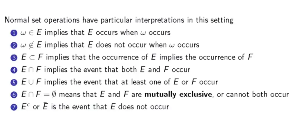
With the basic notation in place, we can perform a series of basic operations such as calculating unions and intersections of events.
The following slide briefly summarizes the most important probability rules.
Properties of Probability Functions
Probabilities can be described as functions of an event where the total probability needs to sum to one. For example, the probability of rolling any number between 1 and six with a fair dice must be one. You’ve covered the entire event space Ω, so you definitely get any one of these numbers. Accordingly, we can describe the probability of the whole event space with the following probability function.
P(Ω) = 1
The probability of rolling an even number E ={2,4,6}, would be 1/2.
P(E) = \frac{1}{2}The complimentary event to E (rolling an odd number) must also be 1/2. The union of E and its complement must sum to 1 and must be mutually exclusive.
P(E) + P(E^c) = 1
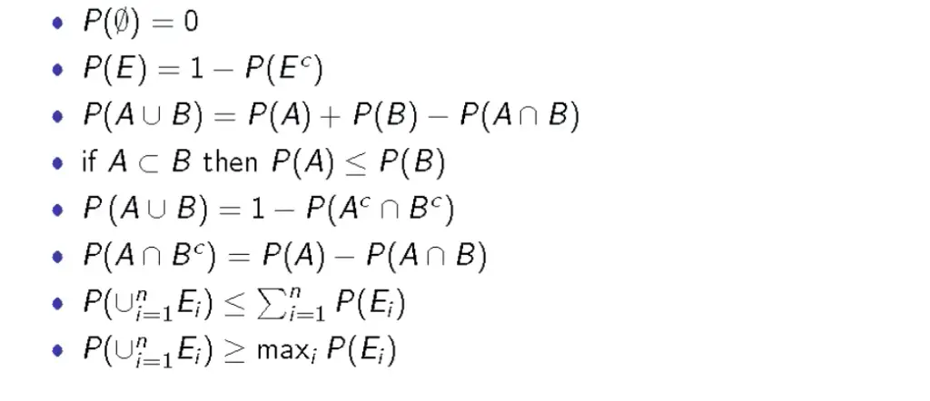
With this knowledge, we can derive the following set of properties that a probability function has to have:
This post is part of a series on statistics for machine learning and data science. To read other posts in this series, go to the index.


