Basic Vector Operations

In this post build a basic understanding of vectors and learn how to perform vector addition, vector subtraction, and vector scaling in a multidimensional space. We also take a brief look at how vectors can be used to construct matrices.
What is a vector?
Every number defines a coordinate along a different dimension in space. For the preceding vector, you would have two dimensions.
\begin{bmatrix}x\\y\end{bmatrix}
that can be plotted on a 2 dimensional grid:

How to add vectors?
Vector addition is performed by taking every entry in the first vector and adding it to the corresponding entry in the second vector. When you add two vectors v1 and v2, the first entry in v1 is added to the first entry in v2, and the second entry in v1 is added to the second entry in v2:
\begin{bmatrix}1\\3\end{bmatrix} + \begin{bmatrix}2\\5\end{bmatrix} = \begin{bmatrix}3\\8\end{bmatrix}How to Subtract Vectors?
Vector subtraction is performed by taking every entry in the first vector and subtracting it from the corresponding entry in the second vector. When you subtract a vector v2 from another vector v1, you deduct the first entry in v2 from the first entry in v1, and you deduct the second entry in v2 from the second entry in v1:
\begin{bmatrix}1\\3\end{bmatrix} - \begin{bmatrix}2\\5\end{bmatrix} = \begin{bmatrix}-1\\-2\end{bmatrix}Scalars
A scalar is a number used to scale a vector. What does this mean in practice?
You take a single number and multiply it with a vector. The number is multiplied with every element, essentially scaling the entire vector by the scalar.
3 \begin{bmatrix}1\\3\end{bmatrix} = \begin{bmatrix}3\\9\end{bmatrix}How can I use this in the real world?
Imagine you run a bakery producing bread, bagels, and donuts. In a typical hour, you sell 40 pieces of bread, 50 bagels, and 30 donuts, netting you a total of $ 250. You can represent this as a vector:
\begin{bmatrix}bread\\bagel\\donut\\total\end{bmatrix}
=
\begin{bmatrix}40\\50\\30\\250\end{bmatrix}
A bread is $3, a bagel $2 and a donut $1.
\begin{bmatrix}bread\\bagel\\donut\\total\end{bmatrix}
=
12
\begin{bmatrix}40\\50\\30\\250\end{bmatrix}
=
\begin{bmatrix}480\\600\\360\\3000\end{bmatrix}
Great, you expect to make 3000 bucks in revenue today.
But wait a minute. Can you really expect people to buy the same ratio of bread, bagels, and donuts every hour?
Of course, you cannot. In the morning, people may be more likely to buy a bagel on the way to work. At lunchtime, they get a donut for dessert, and at night they might do grocery shopping for the family, focusing on bread.
So, simple scalar multiplication is only appropriate for a rough forecast. To gain a more accurate understanding, you need to collect data from previous days and create a new vector representing every item’s exact numbers for every hour of the day.
For the sake of simplicity, let’s add the hours around breakfast, lunch, and dinnertime.
\begin{bmatrix}40\\50\\30\\250\end{bmatrix} + \begin{bmatrix}40\\10\\60\\200\end{bmatrix} + \begin{bmatrix}60\\10\\10\\210\end{bmatrix} =
\begin{bmatrix}140\\70\\100\\660\end{bmatrix}
The number of pieces of bread sold stays constant throughout the day and increases at night, while bagels have a spike in the morning and decline afterward. Donuts see a spike around midday. Revenue is highest in the morning.
That’s the power of vectors. You can represent the relationship between different data items and how they change together.
If you collect the data for several days, a machine learning model can learn these periodic changes in the data and make predictions on your behalf.
To train a machine learning model, you would probably write the three vectors representing the hours together like this:
  \begin{bmatrix}
    40 & 40 & 60  \\
    50 & 10 & 10 \\
    30 & 60 & 10 \\
    250 & 200 & 210 \\
  \end{bmatrix}
You just learned what a matrix is. In its principle, it is nothing but a combination of vectors. But before we can move on to matrixes, we still need to look at some more vector operations.
This post is part of a series on linear algebra for machine learning. To read other posts in this series, go to the index.


