Introduction to the Hypothesis Space and the Bias-Variance Tradeoff in Machine Learning

In this post, we introduce the hypothesis space and discuss how machine learning models function as hypotheses. Furthermore, we discuss the challenges encountered when choosing an appropriate machine learning hypothesis and building a model, such as overfitting, underfitting, and the bias-variance tradeoff.
The hypothesis space in machine learning is a set of all possible models that can be used to explain a data distribution given the limitations of that space. A linear hypothesis space is limited to the set of all linear models. If the data distribution follows a non-linear distribution, the linear hypothesis space might not contain a model that is appropriate for our needs.
To understand the concept of a hypothesis space, we need to learn to think of machine learning models as hypotheses.
The Machine Learning Model as Hypothesis
Generally speaking, a hypothesis is a potential explanation for an outcome or a phenomenon. In scientific inquiry, we test hypotheses to figure out how well and if at all they explain an outcome.
In supervised machine learning, we are concerned with finding a function that maps from inputs to outputs.
But machine learning is inherently probabilistic. It is the art and science of deriving useful hypotheses from limited or incomplete data. Our functions are not axioms that explain the data perfectly, and for most real-life problems, we will never have all the data that exists. Accordingly, we will not find the one true function that perfectly describes the data.
Instead, we find a function through training a model to map from known training input to known training output. This way, the model gradually approximates the assumed true function that describes the distribution of the data.
So we treat our model as a hypothesis that needs to be tested as to how well it explains the output from a given input. We do this using a test or validation data set.
The Hypothesis Space
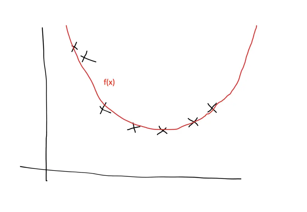
During the training process, we select a model from a hypothesis space that is subject to our constraints. For example, a linear hypothesis space only provides linear models. We can approximate data that follows a quadratic distribution using a model from the linear hypothesis space.

Of course, a linear model will never have the same predictive performance as a quadratic model, so we can adjust our hypothesis space to also include non-linear models or at least quadratic models.
The Data Generating Process
The data generating process describes a hypothetical process subject to some assumptions that make training a machine learning model possible. We need to assume that the data points are from the same distribution but are independent of each other. When these requirements are met, we say that the data is independent and identically distributed (i.i.d.).
Independent and Identically Distributed Data
How can we assume that a model trained on a training set will perform better than random guessing on new and previously unseen data?
First of all, the training data needs to come from the same or at least a similar problem domain. If you want your model to predict stock prices, you need to train the model on stock price data or data that is similarly distributed. It wouldn’t make much sense to train it on whether data.
Statistically, this means the data is identically distributed.
But if data comes from the same problem, training data and test data might not be completely independent. To account for this, we need to make sure that the test data is not in any way influenced by the training data or vice versa. If you use a subset of the training data as your test set, the test data evidently is not independent of the training data. Statistically, we say the data must be independently distributed.
Overfitting and Underfitting
We want to select a model from the hypothesis space that explains the data sufficiently well. During training, we can make a model so complex that it perfectly fits every data point in the training dataset. But ultimately, the model should be able to predict outputs on previously unseen input data. The ability to do well when predicting outputs on previously unseen data is also known as generalization.
There is an inherent conflict between those two requirements.
If we make the model so complex that it fits every point in the training data, it will pick up lots of noise and random variation specific to the training set, which might obscure the larger underlying patterns. As a result, it will be more sensitive to random fluctuations in new data and predict values that are far off. A model with this problem is said to overfit the training data and, as a result, to suffer from high variance.
To avoid the problem of overfitting, we can choose a simpler model or use regularization techniques to prevent the model from fitting the training data too closely. The model should then be less influenced by random fluctuations and instead, focus on the larger underlying patterns in the data. The patterns are expected to be found in any dataset that comes from the same distribution. As a consequence, the model should generalize better on previously unseen data.
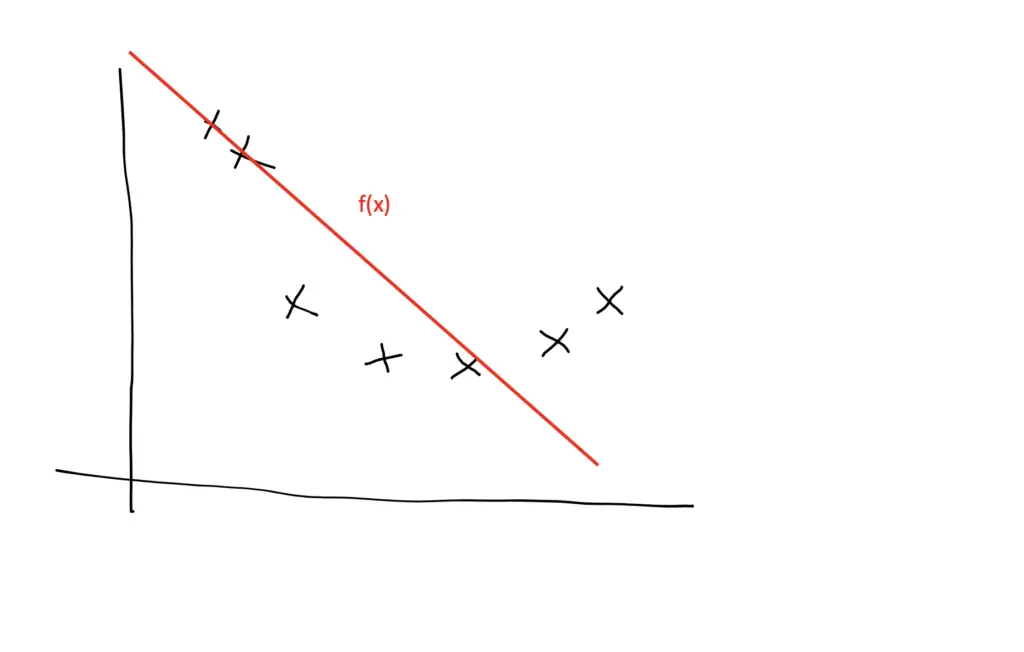
But if we go too far, the model might become too simple or too constrained by regularization to accurately capture the patterns in the data. Then the model will neither generalize well nor fit the training data well. A model that exhibits this problem is said to underfit the data and to suffer from high bias. If the model is too simple to accurately capture the patterns in the data (for example, when using a linear model to fit non-linear data), its capacity is insufficient for the task at hand.
When training neural networks, for example, we go through multiple iterations of training in which the model learns to fit an increasingly complex function to the data.
Typically, your training error will decrease during learning the more complex your model becomes and the better it learns to fit the data. In the beginning, the training error decreases rapidly. In later training iterations, it typically flattens out as it approaches the minimum possible error.
Your test or generalization error should initially decrease as well, albeit likely at a slower pace than the training error. As long as the generalization error is decreasing, your model is underfitting because it doesn’t live up to its full capacity. After a number of training iterations, the generalization error will likely reach a trough and start to increase again. Once it starts to increase, your model is overfitting, and it is time to stop training.
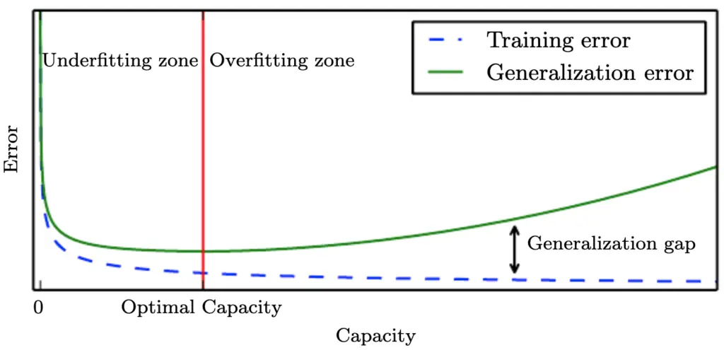
Ideally, you should stop training once your model reaches the lowest point of the generalization error. The gap between the minimum generalization error and no error at all is an irreducible error term known as the Bayes error that we won’t be able to completely get rid of in a probabilistic setting. But if the error term seems too large, you might be able to reduce it further by collecting more data, manipulating your model’s hyperparameters, or altogether picking a different model.
Bias Variance Tradeoff
We’ve talked about bias and variance in the previous section. Now it is time to clarify what we actually mean by these terms.
Understanding Bias and Variance
In a nutshell, bias measures if there is any systematic deviation from the correct value in a specific direction. If we could repeat the same process of constructing a model several times over, and the results predicted by our model always deviate in a certain direction, we would call the result biased.
Variance measures how much the results vary between model predictions. If you repeat the modeling process several times over and the results are scattered all across the board, the model exhibits high variance.
In their book “Noise” Daniel Kahnemann and his co-authors provide an intuitive example that helps understand the concept of bias and variance.
Imagine you have four teams at the shooting range.
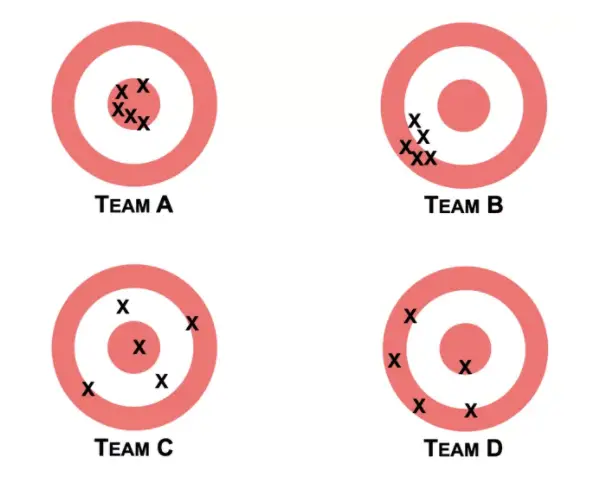
Team B is biased because the shots of its team members all deviate in a certain direction from the center. Team B also exhibits low variance because the shots of all the team members are relatively concentrated in one location.
Team C has the opposite problem. The shots are scattered across the target with no discernible bias in a certain direction.
Team D is both biased and has high variance.
Team A would be the equivalent of a good model. The shots are in the center with little bias in one direction and little variance between the team members.
Generally speaking, linear models such as linear regression exhibit high bias and low variance.
Nonlinear algorithms such as decision trees are more prone to overfitting the training data and thus exhibit high variance and low bias.
A linear model used with non-linear data would exhibit a bias to predict data points along a straight line instead of accomodating the curves. But they are not as susceptible to random fluctuations in the data.
A nonlinear algorithm that is trained on noisy data with lots of deviations would be more capable of avoiding bias but more prone to incorporate the noise into its predictions. As a result, a small deviation in the test data might lead to very different predictions.
To get our model to learn the patterns in data, we need to reduce the training error while at the same time reducing the gap between the training and the testing error. In other words, we want to reduce both bias and variance. To a certain extent, we can reduce both by picking an appropriate model, collecting enough training data, selecting appropriate training features and hyperparameter values.
At some point, we have to trade-off between minimizing bias and minimizing variance. How you balance this trade-off is up to you.
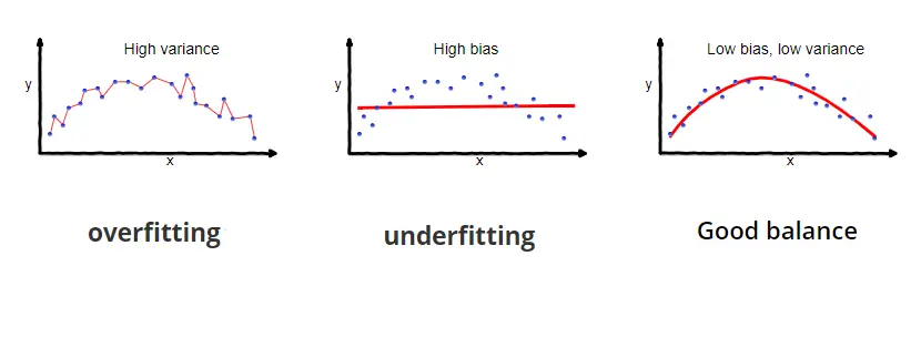
Image taken from https://datacated.com/datacated-challenge/the-bias-and-variance-tradeoff/#page-content
The Bias Variance Decomposition
Mathematically, the total error can be decomposed into the bias and the variance according to the following formula.
Total\; Error = Bias^2 + Variance + Bayes\; Error
Remember that Bayes’ error is an error that cannot be eliminated.
Our machine learning model represents an estimating function \hat f(X) for the true data generating function f(X) where X represents the predictors and y the output values.
Now the mean squared error of our model is the expected value of the squared difference of the output produced by the estimating function \hat f(X) and the true output Y.
MSE(X) = E[(\hat f(X) - Y)^2]
The bias is a systematic deviation from the true value. We can measure it as the squared difference between the expected value produced by the estimating function (the model) and the values produced by the true data-generating function.
Bias(X) = (E[(\hat f(X)] - f(X))^2
Of course, we don’t know the true data generating function, but we do know the observed outputs Y, which correspond to the values generated by f(x) plus an error term.
Y = f(X) + \epsilon
The variance of the model is the squared difference between the expected value and the actual values of the model.
Var(X) = E[(\hat f(X) - E[\hat f(X)])^2 ]
Now that we have the bias and the variance, we can add them up along with the irreducible error to get the total error.
Err(X) = (E[(\hat f(X)] - f(X))^2 +E[(\hat f(X) - E[\hat f(X)])^2 ] + \sigma^2
Summary
A machine learning model represents an approximation to the hypothesized function that generated the data. The chosen model is a hypothesis since we hypothesize that this model represents the true data generating function.
We choose the hypothesis from a hypothesis space that may be subject to certain constraints. For example, we can constrain the hypothesis space to the set of linear models.
When choosing a model, we aim to reduce the bias and the variance to prevent our model from either overfitting or underfitting the data. In the real world, we cannot completely eliminate bias and variance, and we have to trade-off between them.
The total error produced by a model can be decomposed into the bias, the variance, and irreducible (Bayes) error.
