Building a Convolutional Neural Network for Image Classification: A Step-by-Step Example in TensorFlow

In this post, we will learn to build a basic convolutional neural network in TensorFlow and how to train it to distinguish between cats and dogs. We start off with a simple neural network and gradually work our way towards more complex architectures evaluating at each step how the results are changing.
To build this network, I’ve used Google Colab, which lets you train your network on a GPU for free.
Download the Data and Prepare the Dataset
The dataset we are going to use is called cats and dogs. While this dataset can be downloaded directly from TensorFlow, you will need to learn how to import external data if you are serious about deep learning. One of the best places to find training data for your projects is Kaggle. We will obtain the dataset through Kaggle and download it into Google Colab.
If you do not have a Kaggle account, sign up for one. Don’t worry. It is free. Once you’ve signed up, navigate to your account page. There is a small symbol for your profile in the upper right-hand corner from which you can navigate to your account. Once you are there, scroll down to the “API” section and click “Create New API Token”. This will download a Kaggle.json file.

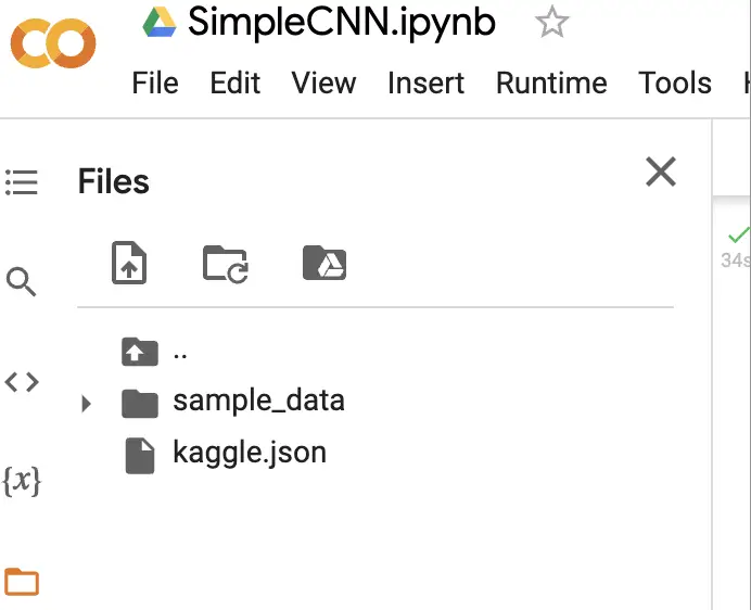
You need to place the Kaggle.json file in your working directory. If you are in Colab, you have a section on the right that gives you an overview of your working directory. Just drag and drop the file in there (note that this will delete the file if you shut down Colab, so you’ll need to re-upload it).
Once the file is in place, you need to install the Kaggle library and move the Kaggle.json file into the directory structure required by Kaggle. This can be achieved with the following commands.
! pip install kaggle
! mkdir ~/.kaggle
! cp kaggle.json ~/.kaggle/
! chmod 600 ~/.kaggle/kaggle.json
Next, you download the cats and dogs dataset into your working directory and unzip it.
! kaggle datasets download chetankv/dogs-cats-images
! unzip dogs-cats-images.zip
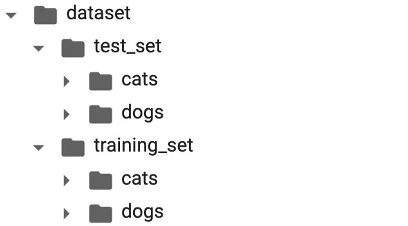
You should now have a directory called dataset in your working directory. Inside the dataset, we have a training set and a test set, each of which contains folders for the images of cats and dogs.
To read the data for our model, we need to define the paths to the images.
train_dir = '/content/dataset/training_set'
train_dir_cats = os.path.join(train_dir,'cats')
train_dir_dogs = os.path.join(train_dir,'dogs')

test_dir = '/content/dataset/test_set'
test_dir_cats = os.path.join(test_dir,'cats')
test_dir_dogs = os.path.join(test_dir,'dogs')
To check that we can import the images correctly, we print the number of images in each directory.
print(len(os.listdir(train_dir_cats))) #4000
print(len(os.listdir(train_dir_dogs))) #4000

print(len(os.listdir(test_dir_cats))) #1000
print(len(os.listdir(test_dir_dogs))) #1000
Import Data with Keras’ ImageDataGenerator
Now it is finally time to import the images and prepare them for training. To do that, we will use the Keras Image data generator. Data generators let you import data from directories, as well as manipulate and preprocess it on the fly.
We first define the image data generators for the training and the test data and tell them what preprocessing steps to perform. In this case, we just want to scale the pixel values to a range from 0 – 1. Pixel values are on a scale from 0 – 255, which is why we divide by 255.
train_generator = ImageDataGenerator(rescale=1./255)

validation_generator = ImageDataGenerator(rescale=1./255)
Now we can import the data through the generator using the “flow_from_directory” method. We also specify in the function call that we want the generator to resize the images to 300×300 pixels and feed them to the models in batches of 32. Since we distinguish between cats and dogs, we have a binary classification problem.
train_generator = ImageDataGenerator(rescale=1./255)
train_generator = train_generator.flow_from_directory(
        train_dir,
        target_size=(300, 300),
        batch_size=32,
        class_mode='binary')


validation_generator = ImageDataGenerator(rescale=1./255)
validation_generator = validation_generator.flow_from_directory(
        test_dir,
        target_size=(300, 300),
        batch_size=32,
        class_mode='binary')
Build a Convolutional Neural Network
When constructing a neural network for image classification, we gradually need to transform our images so that the network can ultimately decide between 2 or more classes.
In convolutional neural networks, you’ll usually achieve this by applying a convolutional layer with several filters to extract features, followed by a pooling layer to summarize features. Both convolutional filters and pooling filters can be used to reduce the dimensionality of the image. This gradually transforms the input image into a feature map where the required features become more prevalent.
In many convolutional neural networks, you’ll often find a pattern where people apply several pairs of convolutional layers followed by pooling layers. The number of filters usually increases in the latter convolutional layers while the input shrinks along the first two dimensions.
In the last part of the network, the input is flattened, and you’ll usually find a few fully connected layers that lead into the output layer, which performs the final classification. To learn more about common convolutional architectures, check out my introduction to convolutional neural network architectures, as well as my post on deep learning architectures for image classification.
First Convolutional Neural Network
We start out with a simple architecture consisting of 2 pairs of convolutional layers and pooling layers. We use a filter size of 3×3 and a ReLU activation for the convolutional layers and a filter size of 2×2 with max-pooling for the pooling layers. All these settings are pretty standard in modern convolutional architectures.
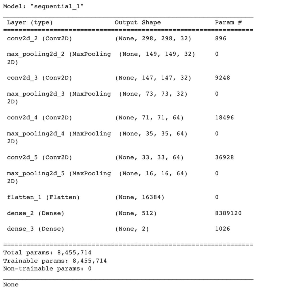
We increase the number of filters from 32 to 64 before flattening the feature map. Lastly, we have another fully connected layer with 512 neurons which leads directly into our output layer with 2 neurons and a sigmoid activation function since we have a binary classification problem (cats vs. dogs). The layers are tied together using Keras’ sequential API.
  model = models.Sequential([
    layers.Conv2D(32, (3,3), activation="relu", input_shape=(300,300, 3)),
    layers.MaxPooling2D((2,2)),
    layers.Conv2D(64, (3,3), activation="relu"),
    layers.MaxPooling2D((2,2)),
    layers.Flatten(),
    layers.Dense(512, activation="relu"),
    layers.Dense(2, activation="sigmoid")
  ])
Then we compile the model using the Adam optimizer and sparse categorical cross-entropy as the loss function and sparse categorical accuracy as the metric.
  model.compile(
      loss= tf.keras.losses.SparseCategoricalCrossentropy(),
      optimizer = optimizers.Adam(),
      metrics = [tf.keras.metrics.SparseCategoricalAccuracy()]
  )
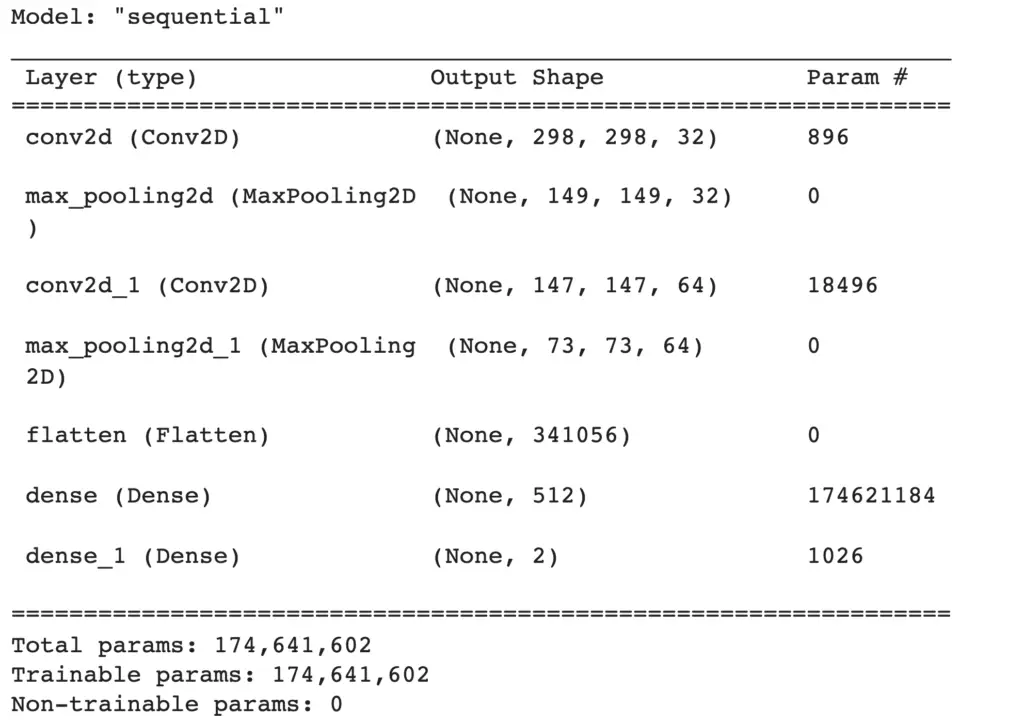
Using the summary function, we can print the model architecture. This is especially useful to check how the dimensionality of the input changes from layer to layer.
print(model.summary())
After investigating the architecture and making sure that it matches our expectations, we finally get to training the neural network. To do that, we call the fit method on the model passing the training and the validation generator for the datasets. In addition, we also tell the function for how many epochs we want to train and how many steps per epoch to use.
history = model.fit(
    train_generator,
    epochs = 20,
    steps_per_epoch = 100,
    validation_data = validation_generator,
    validation_steps = 50
)
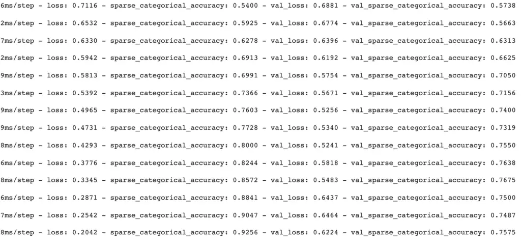
The training will take a while, depending on what hardware you are running the model on. TensorFlow will print the current progress to the console after each epoch.
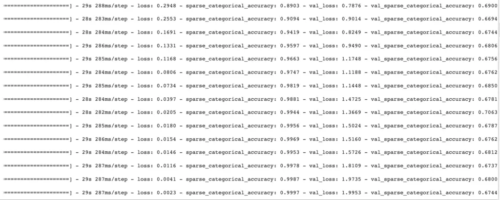
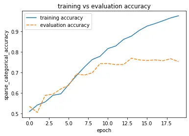
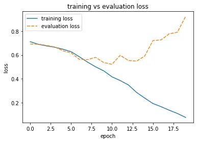
When we look at the output, we can clearly see that something is wrong. The training loss steadily decreases, and the training accuracy increases as expected. However, the validation loss increases while the accuracy increases first to a relatively unimpressive 70% and then starts to decrease.
This looks like the model is overfitting the training data. To get a better overview of what is happening, I’ve defined the following functions to plot the training and validation accuracy.
def get_metrics(history):
  history = history.history
  acc = history['sparse_categorical_accuracy']
  val_acc = history['val_sparse_categorical_accuracy']
  loss = history['loss']
  val_loss = history['val_loss']
  return acc, val_acc, loss, val_loss

def plot_train_eval(history):
  acc, val_acc, loss, val_loss = get_metrics(history)

  acc_plot = pd.DataFrame({"training accuracy":acc, "evaluation accuracy":val_acc})
  acc_plot = sns.lineplot(data=acc_plot)
  acc_plot.set_title('training vs evaluation accuracy')
  acc_plot.set_xlabel('epoch')
  acc_plot.set_ylabel('sparse_categorical_accuracy')
  plt.show()

  loss_plot = pd.DataFrame({"training loss":loss, "evaluation loss":val_loss})
  loss_plot = sns.lineplot(data=loss_plot)
  loss_plot.set_title('training vs evaluation loss')
  loss_plot.set_xlabel('epoch')
  loss_plot.set_ylabel('loss')
  plt.show()
When calling the second function, we get a nice plot.
plot_train_eval(history)
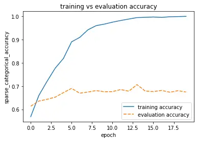
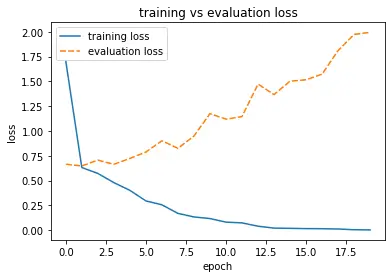
Glancing at the plots, we see immediately that the validation accuracy flatlines right after the first few epochs while the validation loss increases.
Let’s see if we can improve on these results by building a slightly more complicated network. But before we do this, let’s wrap the construction of the first network into a function call so we can easily build it and distinguish it from the other models we are going to build.
def build_model_A():
  model = models.Sequential([
    layers.Conv2D(32, (3,3), activation="relu", input_shape=(300,300, 3)),
    layers.MaxPooling2D((2,2)),
    layers.Conv2D(64, (3,3), activation="relu"),
    layers.MaxPooling2D((2,2)),
    layers.Flatten(),
    layers.Dense(512, activation="relu"),
    layers.Dense(2, activation="sigmoid")
  ])

  model.compile(
      loss= tf.keras.losses.SparseCategoricalCrossentropy(),
      optimizer = optimizers.Adam(),
      metrics = [tf.keras.metrics.SparseCategoricalAccuracy()]
  )

  return model
Second Convolutional Neural Network
The network we’ll build next is essentially a copy of the first network, but we’ve duplicated the first two blocks, each consisting of a convolutional layer and a max-pooling layer. This means we have two convolutional layers with 32 filters followed by max-pooling layers and two convolutional layers with 64 filters followed by max-pooling layers.
def build_model_B():
  model = models.Sequential([
    layers.Conv2D(32, (3,3), activation="relu", input_shape=(300,300, 3)),
    layers.MaxPooling2D((2,2)),
    layers.Conv2D(32, (3,3), activation="relu"),
    layers.MaxPooling2D((2,2)),
    layers.Conv2D(64, (3,3), activation="relu"),
    layers.MaxPooling2D((2,2)),
    layers.Conv2D(64, (3,3), activation="relu"),
    layers.MaxPooling2D((2,2)),
    layers.Flatten(),
    layers.Dense(512, activation="relu"),
    layers.Dense(2, activation="sigmoid")
  ])

  model.compile(
      loss= tf.keras.losses.SparseCategoricalCrossentropy(),
      optimizer = optimizers.Adam(),
      metrics = [tf.keras.metrics.SparseCategoricalAccuracy()]
  )

  return model
When we build the model and evaluate its architecture, we see that the last pooling layer right before we flatten the output produces a feature map of only 16x16x64.
model_2 = build_model_B()
print(model_2.summary())
Early Stopping in TensorFlow
We can tell TensorFlow to stop training early if a certain metric such as the validation accuracy doesn’t improve any further. To stop early, we define a callback and pass it to the fit function before we start to train the model.
early_stopping = tf.keras.callbacks.EarlyStopping(monitor="val_sparse_categorical_accuracy",
                                                  patience=3)

history_b = model_b.fit(
    train_generator,
    epochs = 50,
    steps_per_epoch = 100,
    validation_data = validation_generator,
    validation_steps = 50,
    callbacks= [early_stopping]
)
We’ve set the metric we’d like to monitor to validation accuracy with a patience value of 3. The model will stop training if the validation accuracy hasn’t improved for 3 consecutive epochs.
The accuracy has improved by about 5-6 percentage points. It seems we are on the right path.
Network with Data Augmentation
As the next step, we can add data augmentation to see if it improves our network. When working with images, we can easily multiply our training data by rotating, flipping, or shearing the images. With Keras’ inbuilt data generator, this is easy to implement by simply specifying the transformations we want to perform when instantiating the training data generator.
train_datagen = ImageDataGenerator(rescale=1./255,
        shear_range=0.2,
        zoom_range=0.2,
        horizontal_flip=True)

train_generator = train_datagen.flow_from_directory(
        train_dir,
        target_size=(300, 300),
        batch_size=32,
        class_mode='binary')
We don’t need to perform any augmentation on the validation set since the purpose of augmentation is to provide the network with more variety at training time.
model_b_2 = build_model_B()

early_stopping = tf.keras.callbacks.EarlyStopping(monitor="val_sparse_categorical_accuracy",
                                                  patience=3)

history_b_2 = model_b_2.fit(
    train_generator,
    epochs = 30,
    steps_per_epoch = 100,
    validation_data = validation_generator,
    validation_steps = 50,
    callbacks= [early_stopping]
)
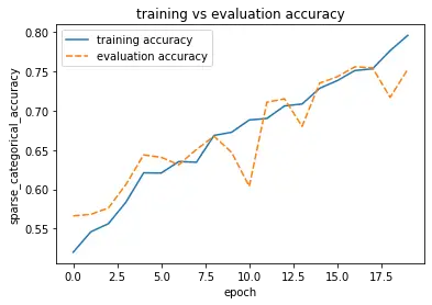
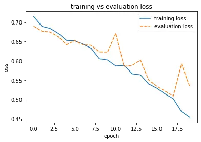
It looks like data augmentation didn’t help increase our validation accuracy and reduce our validation loss particularly. It decreases our training accuracy, which is probably due to the improved image diversity resulting from our data augmentation.
CNN in TensorFlow with Transfer Learning
Rather than building and training our convolutional neural network from scratch, we can import an established model architecture that has been pretrained on another dataset. TensorFlow and Keras make this easy.
We import the InceptionResNetV2 from Tensorflow. This is an advanced convolutional architecture that has been pretrained on more than a million images from the ImageNet database to distinguish between 1000 classes. We specify that we want the pretrained weights from imagenet. Furthermore, we need to pass the input shape and tell the network that we don’t need the top. We will attach the last few layers ourselves so that we can use the network for our dataset.
All of this can be achieved in a single line of code, and TensorFlow will download the model the weights and instantiate InceptionResNet as a base model for us.
base_model = tf.keras.applications.InceptionResNetV2(weights='imagenet', include_top=False, input_shape=(300, 300, 3))
After instantiating the base model, we set the trainable parameter to false. This indicates to TensorFlow that we only want to train the new layers we add but that the pretrained layers should be left untouched. If you have a lot of training data, you may also train the layers of your base model. But in such a simple case as distinguishing between cats and dogs, it would be overkill.
base_model.trainable = False
Now, we can add our own layers and build the model. Essentially, we just want to add the output layer that defines the distinction between two classes instead of 1000 and one or two dense layers to help the network learn. We use the Keras Sequential API and add the layers one by one starting with the layers of the base model. Instead of using a “Flatten” layer, we add a global average pooling layer to transition the output from the format provided by the pretrained model to one that we can use for our fully connected layers.
Global average pooling shrinks the size of the spatial dimensions down to one along all the axes except for the last by averaging according to the last axis. The last axis is usually the number of filters.
I’ve used global average pooling here to introduce the layer, but you can equally use the “Flatten” layer.
The remaining part of the code is very similar to what we’ve used in the previous models. In the last fully connected layer, I’ve used 128 instead of 512 neurons. This choice is due to experimentation. When building a neural network, you often have to find values such as the number of neurons through trial and error.
def build_model_C(base_model):

  model = tf.keras.models.Sequential([base_model])
  model.add(tf.keras.layers.GlobalAvgPool2D())
  model.add(tf.keras.layers.Dense(128,activation='relu'))
  model.add(tf.keras.layers.Dense(2, activation = 'sigmoid'))


  model.compile(
      loss= tf.keras.losses.SparseCategoricalCrossentropy(),
      optimizer = optimizers.Adam(),
      metrics = [tf.keras.metrics.SparseCategoricalAccuracy()]
  )

  return model
We build the model as before.
model_c = build_model_C(base_model)

history_c = model_c.fit(
    train_generator,
    epochs = 20,
    steps_per_epoch = 100,
    validation_data = validation_generator,
    validation_steps = 50
)
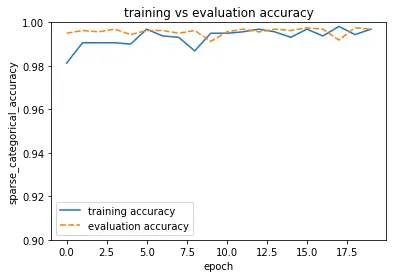
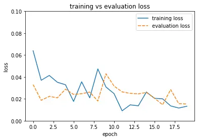
As you may have noticed, I disabled early, stopping to train for the entire 20 epochs. But that would not have been necessary. Both training and validation accuracy hit values >99% after just one epoch and stayed there until the end of training. It seems the pretrained weights were already pretty well attuned to distinguishing between cats and dogs.
Conclusion
There are only very few cases where it makes sense to build and train a neural network from scratch. Whenever you have a use case that involves standard images or objects, I recommend using a pretrained architecture. That way, you can get pretty good performance with only a few hundred or even dozens of pictures at much shorter training times.
This article is part of a blog post series on deep learning for computer vision. For the full series, go to the index.
