Deep Learning Optimization Techniques for Gradient Descent Convergence

In this post, we will introduce momentum, Nesterov momentum, AdaGrad, RMSProp, and Adam, the most common techniques that help gradient descent converge faster.
Understanding Exponentially Weighted Moving Averages
A core mechanism behind many of the following algorithms is called an exponentially weighted moving average. As the name implies, you calculate an average of several observations rather than focusing solely on the most recent observation. For example, suppose you wanted to calculate the moving average of the price p of a certain stock over the past five days.
p = [12.30, 11.00, 10.20, 10.50, 11.10 ]
You take the sum of the last five stock prices per day and divide them by 5.
p_{average} = \frac{12.30+ 11.00+ 10.20+ 10.50+ 11.10}{5} = 11.02Exponentially weighted averages incorporate previous observations in exponentially declining importance in addition to the current one into our estimates.
You need to choose a smoothing parameter β that determines how much weight you give to the current observations as compared to the previous ones. Then you can calculate the exponentially weighted average according to the following formula.
v_{current} = \beta v_{current-1} + (1-\beta) p_{current} The parameter v is the weighted average from the previous step. In our stock price example, we can calculate the moving average from day one and day two. Let’s set β equal to 0.2. Since we are only on day two, the moving average of the first day is equivalent to the price of the first day.
v_{current} = 0.2 \times 12.30 + (1-0.2) \times 11 = 11.26V current is now the moving average of the first two observations. In the next step, we add the third observation and use v current from the previous step.
v_{current} = 0.2 \times 11.26 + (1-0.2) \times 10.20 = 10.41In summary, this process of recursively updating the current v is equivalent to a series in which the contribution of each point p declines exponentially with every timestep.
- On the first day the contribution of p1 to v1 is equivalent to 1.
- On the second day, the contribution of p1 to v2 is equivalent to β
- On the third day, the contribution of p1 to v3 is equivalent to β^2
- On the fourth day, the contribution of p1 to v4 is equivalent to β^3
Since β < 1, we have exponential decline rather than exponential growth.
If we plot the moving average vs. the stock prices over the five days, we see that the average smoothes out the fluctuation in the price.
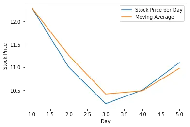
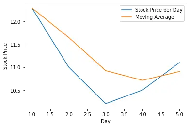
Here we are using an β value of 0.2, which means we give a weight of 80% to the current value while the previous values cumulatively only have a weight of 20%. The smoothing is even more pronounced if we increase the alpha value, thus giving more weight to the previous values. Here is the plot if we give the last values a weight of 50%.
Note that other explanations might multiply the weighted average v with (1-β) and the current value p with β. In this case, β denotes the weight you give to the current value, while in our version, it denotes the weight you give to the weighted average of the previous value. But the principle is the same.
Momentum
Momentum is an optimization technique that helps the gradient descent algorithm converge. Momentum works by incorporating exponentially moving averages of recent observations into the gradient descent update, which helps overcome saddle points in the function space and reduce oscillations due to individual noisy gradients.
Stochastic gradient descent and mini-batch gradient descent tend to oscillate due to the stochasticity that comes from selecting only a small subset of the whole training dataset. The oscillations become especially problematic around local optima, where the cost function tends to have an elongated form.
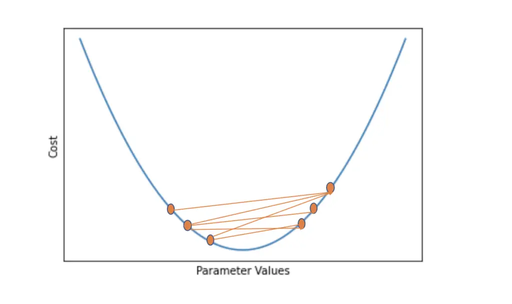
Gradient descent takes much longer to converge and may end up jumping around the local optimum without fully converging. We need a mechanism that makes gradient descent move faster along the elongated side of the cost function and prevents it from oscillating too much. An approach to dampen out the oscillations and make gradient descent move faster along the longer x-axis is to add momentum to the gradient.
It is a bit like pushing a ball down an inclined and slightly bumpy surface. If you let the ball roll down and accelerate on its own, it might jump around a lot more due to all the bumps than if it arrived with some initial velocity. In the latter case, it would be less likely to be thrown off course due to more momentum based on the initial velocity.
We add momentum by adding an exponentially weighted average to the gradient based on the previous gradient values.
Recall the original gradient update rule. You take the derivative of the cost function with respect to the model parameters θ and subtract it from θ multiplied by a learning rate.
In the context of a neural network, theta usually represents the weight and the bias.
\theta_{new} = \theta - \alpha\frac{dJ}{d\theta}We replace the current gradient with a velocity term called v, which represents a sum of the current gradient multiplied by its learning rate and the moving average over the previous gradients multiplied by the parameter β that determines how much weight you assign to the weighted average.
v_{current} = \beta v_{current-1} + \alpha\frac{dJ}{d\theta}Then, we update the parameters θ with the current velocity term instead of the current gradient.
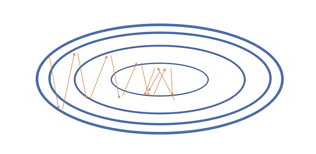
\theta_{current} = \theta _{current-1}- v_{current}Now stochastic gradient descent is more likely to look like in the following illustration with fewer oscillations and a smoother path towards the minimum.
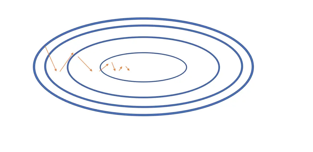
The more successive gradients point in the same direction, gradient descent will develop more momentum in that direction. If the gradients point in different directions, then you will run into more oscillations.
Nesterov Momentum
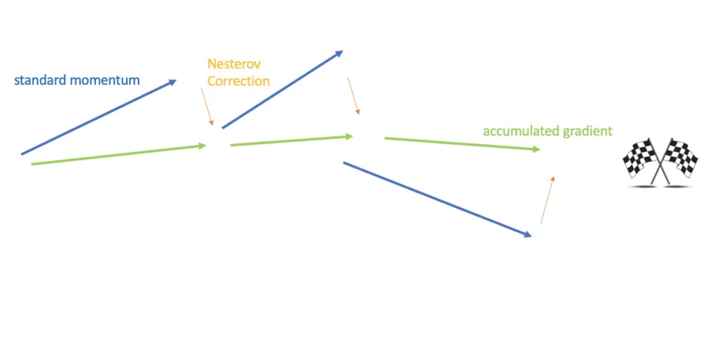
Nesterov momentum is an extension to the momentum algorithm for gradient descent that corrects the trajectory of momentum by incorporating the direction from previously accumulated gradients into the calculation of the current gradient.
Nesterov momentum is an enhancement to the original momentum algorithm that allows gradient descent to look at the next gradient and apply a course correction.
How does this work?
In the original momentum algorithm, we first calculate the gradient with respect to the current θ, and then we add the velocity accumulated from the previous steps.
v_{current} = \beta v_{current-1} + \alpha\frac{dJ}{dθ}
But we know the velocity from the previous time steps before we calculate the gradient of the current time step. Since the next step is a combination of the previous velocity and the current gradient, we already know a large part of what the next step is going to look like. The basic idea of Nesterov momentum is to incorporate this knowledge into the calculation of the next gradient.
Recall that the cost J is a function of the model parameter θ, which is why we can calculate the gradient with respect to θ. In the Nesterov momentum update, we subtract the accumulated velocity from the parameter θ before calculating the gradient.
v_{current} = \beta v_{current-1} + \alpha\frac{dJ(\theta - \beta v_{current-1})}{dθ}Then we apply the standard update.
\theta_{current} = \theta _{current-1}- v_{current}
This has the effect of reigning in the gradient if it veers too much off its trajectory.
AdaGrad
Adagrad is an algorithm that improves the convergence of gradient descent in gently sloped regions of the parameter space by selectively scaling the learning rate based on the magnitude of the gradient.
A common problem with stochastic gradient descent is that it makes very slow progress along flat regions that are common around minima. Since gradient descent usually operates in a high-dimensional space, some dimensions may be flat or almost flat while others are relatively steep. To get gradient descent to converge faster, we want to speed up learning along the flat dimensions while slowing it down along the steeper dimensions.
Since the gradient represents the slope along a given dimension, we expect gradients in gently sloped regions to be relatively small, while those along steeper regions to be large.
Adagrad adjusts the learning rate by a factor including the inverse of the sum of the squared gradients up to that point in time. This ensures that the learning rate is smaller for parameters with large accumulated gradients while it is larger for parameters with small accumulated gradients.
The exact update rule is
\theta_{new} = \theta_t - \frac{\alpha}{\sqrt{G_t + \epsilon}}g_twhere g represents the gradient of the loss function with respect to θ at the current time step t.
g_t = \frac{dJ}{d\theta_t}The parameter epsilon is a small constant to prevent division by 0.
Note that the gradient is a vector containing the gradients with respect to all the parameters. If we have a number k parameters, the vector is of length k.
Capital G is a matrix that represents the outer product over all gradient vectors for the previous time steps up to the current time step t.
G_t = \sum^t_{i=i} g_t g_t^T \; where\; G_t \in \mathbb{R}^{K \times K}Since g is of length k, we end up with a matrix G of dimensionality equal to k times k.
For each individual gradient out of the k gradients, G is a sparse matrix where the diagonal elements represent the sum of the squared gradient with respect to the parameter θ_k.
\begin{bmatrix}
G_t^{(1,1)} & 0  & ... & 0 \\
0 & G_t^{(2,2)} & ...&0 \\
: & : & : & : \\
0 & 0 & ... &  G_t^{(k,k)}
\end{bmatrix}
RMSProp
A common problem with Adagrad is that the gradients will accumulate, leading the learning rate to continue to decay with every timestep, which will ultimately slow down learning.
RMSProp is an optimization algorithm for gradient descent that aims to mitigate the problem of decaying learning rates by using a weighted average over previous gradients.
Like in the momentum algorithm, we maintain an exponentially weighted average of the gradient.
a_{t} = \beta a_{t-1} + (1 - \beta) \frac{dJ}{d\theta_t}Instead of a constantly growing accumulated gradient, this gives us a term where older gradients gradually lose their value as new gradients are added. Contrary to Adagrad, we use this weighted average to modify the learning rate in the update equation.
\theta_{new} = \theta_t - \frac{\alpha}{\sqrt{a_t + \epsilon}}\frac{dJ}{d\theta_t}Adam Optimization
Adam is an optimization algorithm for gradient descent-based learning methods that selectively adapts the learning rates for individual parameters and incorporates the mean as well as the uncentered variance of the gradient into the parameter update. Adam stands for adaptive moment estimation.
Adam calculates weighted averages of the gradients as well as the squared gradients up to the current time step t. The variable m_t is an estimate of the mean of the gradients up to this point (the first moment).
m_{t} = \beta_1 m_{t-1} + (1 - \beta_1) \frac{dJ}{d\theta_t}The variable v_t is an estimate of the uncentered variance of the gradients up to this point (the second moment).
v_{t} = \beta_2 v_{t-1} + (1 - \beta_2) (\frac{dJ}{d\theta_t})^2Next, we need to bias correct these estimates. The reason for the bias correction is that the initial expressions for v and m are equal to 0. Since β1 αnd β2 are typically set to values close to 1 (such as β1=0.9 αnd β2=0.999), the updates to v and m will be extremely small. As a result, learning will initially be very slow. The bias correction is applied as follows.
\hat m = \frac{m_t}{1-\beta_1}\hat v = \frac{v_t}{1-\beta_2}As in RMSProp, we use the term weighted average of the squared gradient to adaptively scale the learning rate. Like in momentum, we use the weighted average of the past gradients instead of the current gradient. In both cases, we additionally use bias correction.
\theta_{new} = \theta_t - \frac{\alpha}{\sqrt{\hat v_t + \epsilon}} \hat m_tThe Adam algorithm has empirically proven to be very successful in the training of deep neural networks. Accordingly, it has become very popular in the deep learning community.
This article is part of a blog post series on the foundations of deep learning. For the full series, go to the index.
