Deep Learning for Semantic Image Segmentation: A Worked Example in TensorFlow

In this post, we will develop a practical understanding of deep learning for image segmentation by building a UNet in TensorFlow and using it to segment images.
What is Image Segmentation?
Image Segmentation is a technique in digital image processing that describes the process of partitioning an image into sections. Often the goal is to identify and extract specific shapes of interest in an image.
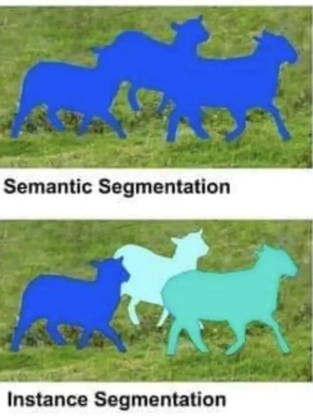
When extracting shapes from images, we distinguish between instance segmentation and semantic segmentation.
What is Semantic Segmentation?
Semantic segmentation attempts to find all objects of a certain category while treating them as one entity within the image. For example, a program that identifies the shapes of several dogs within an image without distinguishing between individual dogs is doing semantic segmentation.
What is Instance Segmentation?
Instance segmentation attempts to extract the shape of objects from an image while distinguishing between individual instances of multiple objects within the same category. A program that identifies several dogs within an image and treats each dog as a separate instance instead of as a part of one entity is performing instance segmentation.
Neural networks have emerged as one of the most promising techniques in image segmentation. In the following tutorial, we will train a neural network to perform semantic segmentation by distinguishing between background, object boundary, and object of interest.
What is a UNet?
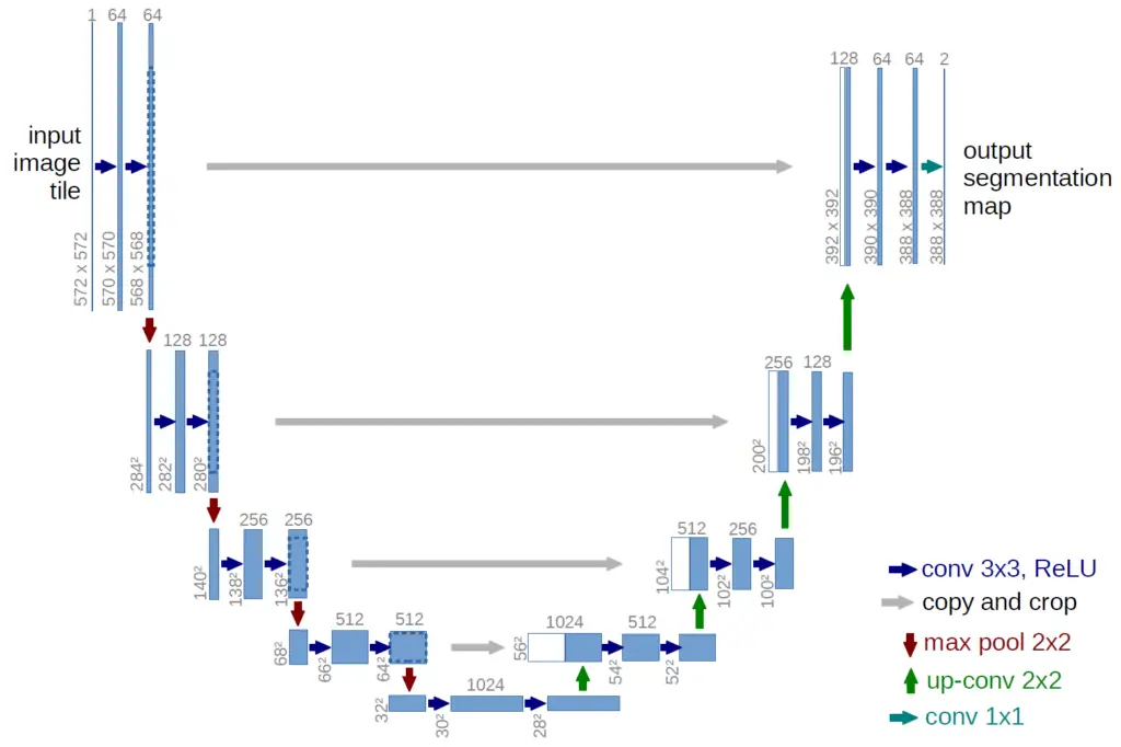
The UNet is a convolutional neural network architecture developed for image segmentation. The first part of the network consists of an encoder that reduces the spatial information while extracting feature information through a series of convolutional layers and ReLU activation functions. The encoder is followed by a decoder that constructs a mask of the objects from the encoding in the original size of the input image.
UNet was created by Olaf Ronneberger, Philipp Fischer, and Thomas Brox at the University of Freiburg in Germany.
Getting Set Up
To follow the tutorial, you’ll need to open a Jupyter Notebook and have TensorFlow installed. If you don’t already have these tools installed, I suggest creating a new virtual environment with anaconda or pip and installing the jupyter-notebook, tensorflow, numpy, matplotlib, scikit-image, os, and random packages into that environment.
The TensorFlow installation will automatically include Keras. I’ve used Keras 2.7.0 when writing this tutorial. If you use another version, you might run into errors. To be on the safe side, I suggest running “pip install keras==2.7.0” before you continue with the tutorial.
As an alternative, you can check out Google Colab. Colab is especially interesting if you don’t have a GPU available for training on your local machine. Up to a certain time limit, you can train on GPU for free on Colab.
Next, you can import these packages as follows.
import os
import random


import numpy as np
import tensorflow as tf
from tensorflow import keras

from keras.preprocessing.image import load_img, array_to_img, img_to_array
from keras.models import Model, load_model
from keras.layers import Input, Activation, SeparableConv2D, BatchNormalization, UpSampling2D
from keras.layers.core import Dropout, Lambda
from keras.layers.convolutional import Conv2D, Conv2DTranspose
from keras.layers.pooling import MaxPooling2D
from keras.layers.merge import concatenate
from keras.callbacks import EarlyStopping, ModelCheckpoint

from skimage.io import imshow

import matplotlib.pyplot as plt
%matplotlib inline
Download and Prepare the Data
We will rely on the Oxford Pets dataset to build our model. You’ll find the data here (on Kaggle). Hit the download button and move the folder into your working directory (you probably will have to sign in to Kaggle before you can download). Inside you’ll find several nested folders. We need the “images” folder that should contain 7390 jpg images of various pets and the “trimaps” folder that contains the segmentation masks corresponding to the pet images.
I’ve arranged the data folders as follows in my working directory:
input_dir = 'pets/pets_images'
target_dir = 'pets/pets_annotations/trimaps'
Next, we create a sorted list with all the image paths so that we can import the images and their corresponding segmentation masks in parallel.
input_img_paths = sorted(
    [
        os.path.join(input_dir, fname)
        for fname in os.listdir(input_dir)
        if fname.endswith(".jpg")
    ]
)
target_img_paths = sorted(
    [
        os.path.join(target_dir, fname)
        for fname in os.listdir(target_dir)
        if fname.endswith(".png") and not fname.startswith(".")
    ]
)
Before we can feed the data to the neural network, we need to ensure the images all have the same size. Therefore, we define a standard size of 256×256. The pictures of the animals are standard RGB images and have three channels, while the masks only have one channel. We are setting the segmentation task up as a classification problem in which the network should learn to classify the pixels into one of 3 classes (background, object boundary, object).
IMG_WIDTH_HEIGHT = 256
IMG_CHANNELS = 3
classes = 3
We define two empty vectors of zeros that we then fill with the images and masks as we import and resize them.
X = np.zeros((len(input_img_paths), IMG_WIDTH_HEIGHT, IMG_WIDTH_HEIGHT, 3), dtype=np.float32)
Y = np.zeros((len(input_img_paths), IMG_WIDTH_HEIGHT, IMG_WIDTH_HEIGHT, 1), dtype=np.uint8)


for i in range(len(input_img_paths)):
    img_path = input_img_paths[i]
    img = load_img(img_path, grayscale=False,target_size=(IMG_WIDTH_HEIGHT, IMG_WIDTH_HEIGHT)) #imread(img_path)[:,:,:3] #.astype("float32") #/ 255.0 -> is done by rgb2gray
    img = img_to_array(img)
    X[i] = img.astype('float32') / 255.0

    mask_path = target_img_paths[i]
    mask = load_img(mask_path, grayscale=True,target_size=(IMG_WIDTH_HEIGHT, IMG_WIDTH_HEIGHT)) #imread(img_path)[:,:,:3] #.astype("float32") #/ 255.0 -> is done by rgb2gray
    mask = img_to_array(mask)
    Y[i] = mask
Note that we divide the image data by 255. We do this because pixel values in a standard RGB image range from 0-255. To enable the network to learn faster, we want all the values to be on a scale between 0 and 1. To accommodate a huge range of values between 0 and 1, we convert the values to 32Bit encoded floating-point numbers. In the case of the mask, we only have three values (0, 1, and 2). These correspond nicely to the three classes between which we want to distinguish. Accordingly, no division by 255 is necessary, and 8Bit integer encoding is sufficient.
As the last step in our data preparation, we split the data into a training and a testing set using 80% of the samples for training and 20% for testing.
train_test_split = int(len(input_img_paths)*0.8)
X_train = X[:train_test_split]
Y_train = Y[:train_test_split]

X_test = X[train_test_split:]
Y_test = Y[train_test_split:]
As a sanity check, let’s visualize a randomly selected sample and its corresponding mask from the training data.
i = random.randint(0, len(X_train))
print(i)
imshow(X_train[i])
plt.show()
imshow(np.squeeze(Y_train[i]))
plt.show()
Building a UNet in TensorFlow
If we have a look at the UNet architecture diagram above, we see that the contracting path follows a pattern. There are always two convolutional layers with ReLU activation functions followed by a Max Pooling layer that reduces the vertical and horizontal image dimensions by half while expanding the third dimension.
We can implement this functionality in a Python function that takes the feature map from the previous layer as an input. If it is the first layer, we pass in the image. Furthermore, we pass the number of filters (you might want to change the number of filters if the dimensions of your input change). The dropout probability allows us to implement an additional dropout layer for regularization. Lastly, we have a boolean flag indicating whether we want to apply max pooling.
def convolutional_block(inputs=None, n_filters=32, dropout_prob=0, max_pooling=True):

    conv = Conv2D(n_filters,
                  kernel_size = 3,
                  activation='relu',
                  padding='same',
                  kernel_initializer=tf.keras.initializers.HeNormal())(inputs)
    conv = Conv2D(n_filters,
                  kernel_size = 3,
                  activation='relu',
                  padding='same',
                  kernel_initializer=tf.keras.initializers.HeNormal())(conv)


    if dropout_prob > 0:
        conv = Dropout(dropout_prob)(conv)

    if max_pooling:
        next_layer = MaxPooling2D(pool_size=(2,2))(conv)


    else:
        next_layer = conv

    #conv = BatchNormalization()(conv)
    skip_connection = conv

    return next_layer, skip_connection
Inside the function, we have two convolutional layers with a kernel size of 3. Then we optionally activate the dropout layer and the Max Pooling layer depending on the parameters we’ve passed to it. The max-pooling layer uses a kernel size of 2×2, which reduces the feature map by 1/2 along the horizontal and vertical dimensions. In a UNet, we employ skip connections, which means that we want to preserve the feature map before pooling and pass it to the corresponding upsampling block. Accordingly, we save the feature map to a variable called skip connection, without the pooling applied to it.
Similarly, we can summarize the steps in the expansive part in a function. The expansive part performs a series of upsampling operations that basically reverse the convolutions and reconstruct the original image. As input, we pass the output from the preceding layer and the skip connection from the corresponding downsampling block. The horizontal arrows in the diagram nicely illustrate how the skip connections travel. Lastly, we also pass the number of filters.
def upsampling_block(expansive_input, contractive_input, n_filters=32):

    up = Conv2DTranspose(
                 n_filters,
                 kernel_size = 3,
                 strides=(2,2),
                 padding='same')(expansive_input)

    merge = concatenate([up, contractive_input], axis=3)
    conv = Conv2D(n_filters,
                 kernel_size = 3,
                 activation='relu',
                 padding='same',
                 kernel_initializer=tf.keras.initializers.HeNormal())(merge)
    conv = Conv2D(n_filters,
                 kernel_size = 3,
                 activation='relu',
                 padding='same',
                 kernel_initializer=tf.keras.initializers.HeNormal())(conv)

    return conv
First, we perform the inverse of the convolutions and max-pooling operations on the input we receive from the preceding block using the Conv2DTranspose layer with a filter size of 3×3 and a stride of 2×2. Now, the input should have the same dimensions as the skip connection we received from the contractive block. This means that we can concatenate them before pushing the combined output through 2 convolutional layers to extract the features for the final mask we want to produce.
Lastly, we can construct our UNet in a new function using the functions defined above. As input, we require the dimensions of the input image, along with the number of filters and the number of classes we want to distinguish between.
def unet_model(input_size=(IMG_WIDTH_HEIGHT, IMG_WIDTH_HEIGHT
                           , IMG_CHANNELS), n_filters=32, n_classes=3):

    inputs = Input(input_size)

    #contracting path
    cblock1 = convolutional_block(inputs, n_filters)
    cblock2 = convolutional_block(cblock1[0], 2*n_filters)
    cblock3 = convolutional_block(cblock2[0], 4*n_filters)
    cblock4 = convolutional_block(cblock3[0], 8*n_filters, dropout_prob=0.2)
    cblock5 = convolutional_block(cblock4[0],16*n_filters, dropout_prob=0.2, max_pooling=None)

    #expanding path
    ublock6 = upsampling_block(cblock5[0], cblock4[1],  8 * n_filters)
    ublock7 = upsampling_block(ublock6, cblock3[1],  n_filters*4)
    ublock8 = upsampling_block(ublock7,cblock2[1] , n_filters*2)
    ublock9 = upsampling_block(ublock8,cblock1[1],  n_filters)

    conv9 = Conv2D(n_classes,
                 1,
                 activation='relu',
                 padding='same',
                 kernel_initializer='he_normal')(ublock9)

    #conv10 = Conv2D(n_classes, kernel_size=1, padding='same', activation = 'softmax')(conv9)
    conv10 = Activation('softmax')(conv9)

    model = tf.keras.Model(inputs=inputs, outputs=conv10)

    return model
The standard UNet architecture cuts the horizontal and vertical dimensions in half while doubling the filter dimensions in every contractive block. In addition, we apply dropout to the last two blocks and suspend pooling in the last block since no further dimensionality reduction is required according to the architecture diagram. The upsampling blocks should be self-explanatory.
After the upsampling, we use a convolutional layer with a 1×1 kernel size and a softmax activation function to produce the classification of the pixels into one of the three classes. If we only had two classes you could also use the sigmoid activation function.
Lastly, we need to combine everything into a Keras model. Thanks to the Keras functional API, this is as simple as passing the input and the expected output.
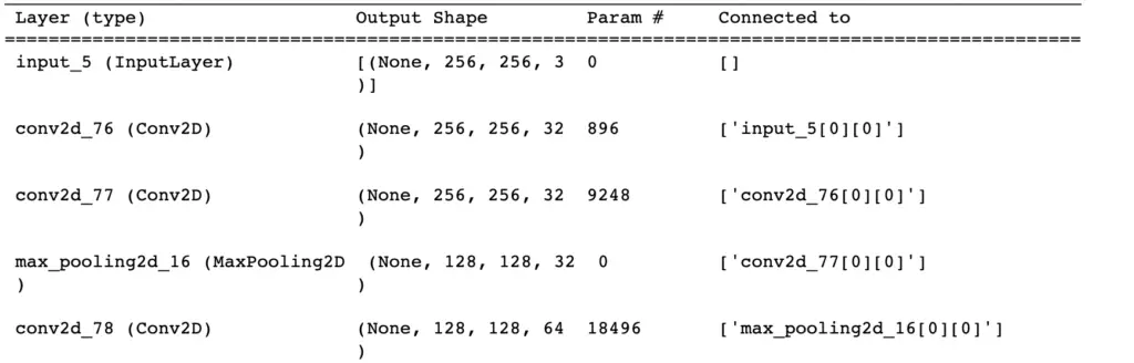
Let’s initialize the network and look at the summary as a sanity check. You should get a nice summary that approximately looks like the following. Note that I’ve only printed the beginning and that your layer numbers will likely be different. The most important thing is that the dimensions in the output shape match your expectations.
unet = unet_model((IMG_WIDTH_HEIGHT, IMG_WIDTH_HEIGHT, IMG_CHANNELS), n_classes=3)
unet.summary()
We are finally ready to compile our model and start to train it.
EPOCHS = 30

unet.compile(optimizer='adam', loss='sparse_categorical_crossentropy', metrics=['accuracy'])

earlystopper = EarlyStopping(patience=5, verbose=1)
model_history = unet.fit(X_train, Y_train, validation_split=0.1, batch_size=16, epochs=EPOCHS, callbacks=[earlystopper])
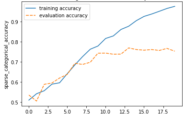
When compiling, make sure you use sparse categorical cross-entropy. If we had a binary classification problem, we could also use binary cross-entropy. Adam is generally a good default optimizer but feel free to play around with others. I decided to train for 30 epochs with an early stopping callback in case the accuracy stops improving earlier. My validation accuracy tops out at approximately 83%.
That is enough for our purpose. Now, we can use the model to create segmentation masks for our test data.
predictions = unet.predict(X_test)
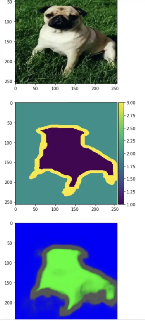
As a sanity check and to see how our hard work has paid off, we can visualize a random image, its corresponding mask, and the prediction generated by the model.
i = 1
imshow(X_test[i])
plt.show()
imshow(np.squeeze(Y_test[i]))
plt.show()
imshow(np.squeeze(predictions[i]))
plt.show()
This article is part of a blog post series on deep learning for computer vision. For the full series, go to the index.
