Understanding Backpropagation With Gradient Descent

In this post, we develop a thorough understanding of the backpropagation algorithm and how it helps a neural network learn new information. After a conceptual overview of what backpropagation aims to achieve, we go through a brief recap of the relevant concepts from calculus. Next, we perform a step-by-step walkthrough of backpropagation using an example and understand how backpropagation and gradient descent work together to help a neural network learn.

Backpropagation is an algorithm used in machine learning that works by calculating the gradient of the loss function, which points us in the direction of the value that minimizes the loss function. It relies on the chain rule of calculus to calculate the gradient backward through the layers of a neural network. Using gradient descent, we can iteratively move closer to the minimum value by taking small steps in the direction given by the gradient.

In other words, backpropagation and gradient descent are two different methods that form a powerful combination in the learning process of neural networks.
For the rest of this post, I assume that you know how forward propagation in a neural network works and have a basic understanding of matrix multiplication. If you don’t have these prerequisites, I suggest reading my article on how neural networks learn.

Why We Need Backpropagation

During forward propagation, we use weights, biases, and nonlinear activation functions to calculate a prediction y hat from the input x that should match the expected output y as closely as possible (which is given together with the input data x). We use a cost function to quantify the difference between the expected output y and the calculated output y hat.

J = \frac{1}{n} \sum_{i=1}^{n} L(\hat y, y)

The goal of backpropagation is to adjust the weights and biases throughout the neural network based on the calculated cost so that the cost will be lower in the next iteration. Ultimately, we want to find a minimum value for the cost function. But how exactly does that work?

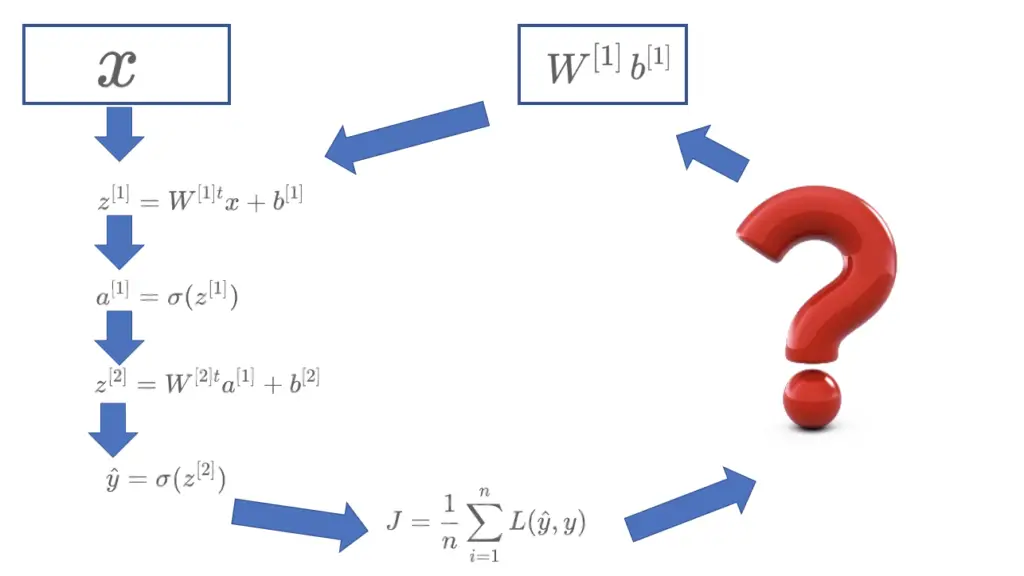
The adjustment works by finding the gradient of the cost function through the chain rule of calculus.

Calculus For Backpropagation

With calculus, we can calculate how much the value of one variable changes depending on the change in another variable. If we want to find out how a change in a variable x by the fraction dx affects a related variable y, we can use calculus to do that. The change dx in x would change y by dy.

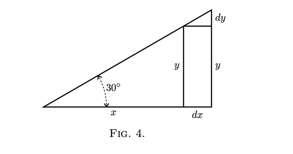
In Calculus notation, we express this relationship as follows.

\frac{dy}{dx}

This is known as the derivative of y with respect to x.

The first derivative of a function gives you the slope of that function at the evaluated coordinate. If you have functions with several variables, you can take partial derivatives with respect to every variable and stack them in a vector. This gives you a vector that contains the slopes with respect to every variable. Collectively the slopes point in the direction of the steepest ascent along the function. This vector is also known as the gradient of a function. Going in the direction of the negative gradient gives us the direction of the steepest descent. Going down the route of the steepest descent, we will eventually end up at a minimum value of the function.

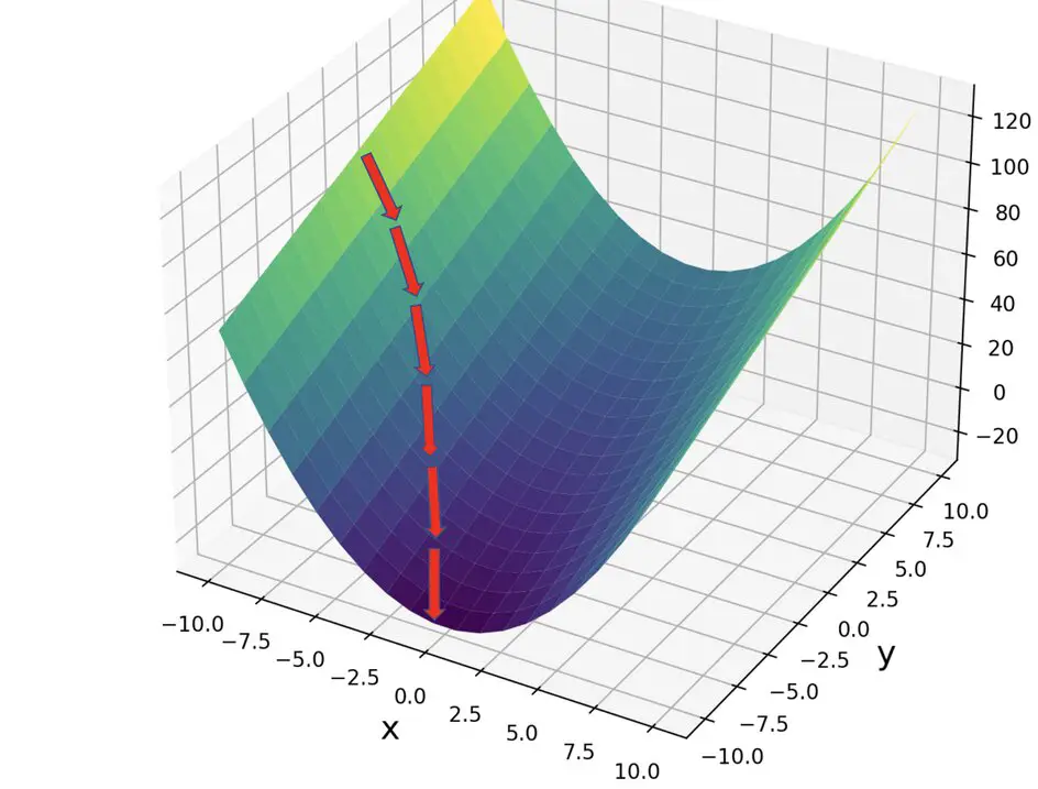
For a more thorough explanation of derivatives as slopes, partial derivatives, and gradients, check out my series of posts on calculus for machine learning.

Backpropagation: Error Calculation and Weight Adjustment

In a neural network, we are interested in how the change in weights affects the error expressed by the cost J. Our ultimate goal is to find the set of weights that minimizes the cost and thus the error. Thus, our intermediate goal is to find the negative gradient of the cost function with respect to the weights, which points us in the direction of the desired minimum.

-\frac{dJ}{dW}

Let’s look at a concrete example with two layers, where each layer has one neuron. For the sake of simplicity, we will ignore the bias b for now.
We need to calculate the derivatives of the cost J with respect to w2 and w1 and update the respective weights by the derivative term by going back through the network.

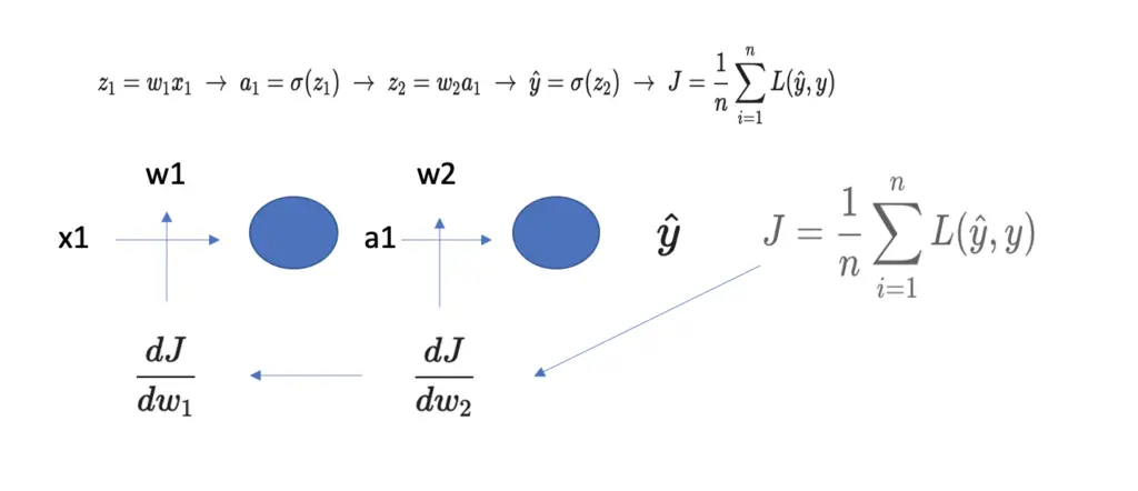
But w2 and w1 are not directly related to the cost. To get to them, we have to differentiate through intermediate functions such as the activations computed by the neurons.

Calculating the Adjustment to W2

J is related to w2 through the following equations in the forward pass.

 z_2 = w_2 a_1 \;  \rightarrow \; \hat y = \sigma(z_2) \;  \rightarrow \; J = \frac{1}{n} \sum_{i=1}^{n} L(\hat y, y)

The backward differentiation through several intermediate functions is done using the chain rule.

\frac{dJ}{dw_2}  = \frac{dJ}{d\hat y} \frac{d\hat y}{ dz_2}  \frac{ dz_2} {dw_2}

The derivative of J with respect to w2 gives us the value by which to adjust the weight w2.

Note: You might also see versions of this formula that use the partial differentiation symbol instead of the d.

\frac{\partial J}{\partial w_2}  = \frac{\partial J}{\partial  \hat y} \frac{\partial  \hat y}{ \partial 
 z_2}  \frac{ \partial  z_2} {\partial  w_2}

The partial derivative is the correct sign in functions where you have multiple variables that can vary. For example, if you have a vector of many weights, you would use the partial derivative symbol. But to avoid unnecessary confusion, we will stick with the d notation throughout this post.

Calculating the Error and Evaluating the Derivatives

Conceptually we now know what derivatives to evaluate and how to chain them together to get the desired weight adjustment. In this subsection, we will evaluate the derivatives. For implementing neural networks with a framework like TensorFlow or Pytorch, the conceptual understanding is sufficient. So feel free to skip ahead to the next section if you are not interested in the nitty-gritty math.

First, we have to evaluate the derivative of the cost J with respect to y hat.

The cost is the average loss over all training examples.

J(W, b) = \frac{1}{n} \sum_{i=1}^{n} L(\hat y_i, y_i)

We use the cross-entropy loss to calculate the difference between predicted and expected values.

L(\hat y, y) = -(y \; log(\hat y) + (1-y)log(1-\hat y))

So the derivative of the cost looks as follows:

 \frac{dJ}{d \hat y} =  \frac{d}{d \hat y} \left( \frac{1}{n} \sum_{i=1}^{n} -(y \; log(\hat y) + (1-y)log(1-\hat y)) \right)

=  - \frac{d}{d \hat y} \left[ y \; log(\hat y) + (1-y)log(1-\hat y) \right]

 \frac{dJ}{d \hat y} =\frac{y}{\hat y} + \frac{1-y}{1- \hat y}

Next, we need to evaluate the derivative of the predicted outcome y hat with respect to z_2, the value fed to the last sigmoid activation.

\frac{d\hat y}{ dz_2} = \frac{d}{ dz_2} \sigma(z_2) = \frac{d}{ dz_2} (\frac{1}{1 + e^{z_2}})

\frac{d\hat y}{ dz_2}  = \sigma(z_2)(1-\sigma(z_2)) =  \frac{1}{1 + e^{z_2}}( 1 -  \frac{1}{1 + e^{z_2}})

Finally, we evaluate the derivative of z_2 with respect to the weight w_2.

\frac{ dz_2} {dw_2} = \frac{ d} {dw_2} (w_2a_1) = a_1

Combining it all, we get the following expression for the derivative of the cost with respect to w_2-

\frac{dJ}{dw_2}  = \frac{dJ}{d\hat y} \frac{d\hat y}{ dz_2}  \frac{ dz_2} {dw_2} = (\frac{y}{\hat y} + \frac{1-y}{1- \hat y}) [\sigma(z_2)(1-\sigma(z_2))] a_1

Calculating the Adjustment to W1

To adjust w1, we can follow the same principle, but we have to go back even further.

z_1=w_1x_1 \; \rightarrow \;  a_1=\sigma(z_1)\; \rightarrow \; z_2 = w_2 a_1 \;  \rightarrow \; 

\hat y = \sigma(z_2) \;  \rightarrow \; J = \frac{1}{n} \sum_{i=1}^{n} L(\hat y, y)

This gives us the following backward pass.

\frac{dJ}{dw_1}  = \frac{dJ}{d\hat y} \frac{d\hat y}{ dz_2} \frac{ dz_2} {da_1}\frac {da_1}{ dz_1} \frac {dz_1}{ dw_1}

I’ll leave the differentiation as an exercise to you. We’ve already evaluated the first two derivatives in the chain in the previous section. So you just have to evaluate the last three elements in the chain based on the equations above.

Adjusting the Weights with Gradient Descent

Once we have calculated the gradient of J with respect to w2 using the chain rule, we can subtract it from the original weight w2 to move in the direction of the minimum value of the cost function. But in a non-linear function, the gradient will be different at every point along the function. Therefore, we can’t just calculate the gradient once and expect it to lead us straight to the minimum value. Instead, we need to take a very small step in the direction of the current gradient, recalculate the gradient based on the new location, take a step in that direction, and repeat the process.

In fact, subtracting the gradient as-is from the weight will likely result in a step that is too big. Before subtracting, we therefore multiply the derivative with a small value α called the learning rate. If we don’t use this learning rate, the weights are manipulated too quickly and the network won’t learn properly.

w_{2new} = w_2 - \alpha\frac{dJ}{dw_2}

Similarly, we perform the weight adjustment on w_1:

w_{1new} = w_1 - \alpha\frac{dJ}{dw_1}

We repeat this process many times over until we find a local minimum.

A Note on Backpropagation in Practice

Note that this is a highly simplified calculation. In a fully connected neural network, you would have several neurons in each layer, and each neuron would connect to each neuron in the next layer. When going back, you have to calculate the derivative of each connection to the next layer and add them all up to attain the correct weight adjustment term.

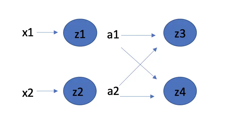
\frac{d z_4}{d a_1} + \frac{d z_3}{d a_1}

Luckily, you won’t ever have to do this by hand. Deep learning frameworks take care of it for you. Understanding the general principles of backpropagation at the level of detail discussed here is sufficient for a practitioner.

This article is part of a blog post series on the foundations of deep learning. For the full series, go to the index.