What is the Law of Large Numbers

In this post, we introduce the law of large numbers and its implications for the expected value and the variance.

The law of large numbers states that the larger your sample size the closer your observed sample mean is to the actual population mean. Intuitively this makes sense.

Suppose, you wanted to estimate the distribution of heights in a country, Measuring the heights of 1000 people from that country is going to give you a better estimate of the mean than measuring the heights of 100 people.

If you throw a fair 6-sided dice, you would expect to throw an average value of 3.5. The expected value of your random variable X that models the distribution of dice throws would be 3.5

E(X) = \frac{1+2+3+4+5+6}{6} = 3.5

But with one single trial, it could be any value between 1 and 6. In fact, 3.5 would be impossible with a single trial. If you cast the dice n times where n is a large number, it is much more likely that you obtain an average of 3.5.

\bar X_n =  \frac{x_1,x_2,...x_n}{n}

We can show this graphically. The following plot shows the mean of 500 samples, each consisting of an increasing number of dice throws. We start with a sample containing one throw and end with a sample of 500 throws.

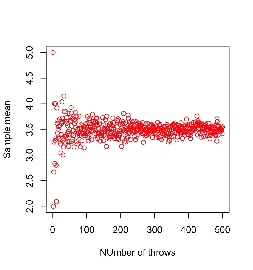
As we can see, the sample mean converges to 3.5 as the number of throws in the sample increases.

Weak Law of Large Numbers

This observation is formalized in the weak law of large numbers, which states that the sample average converges in probability towards the expected value.

\lim_{n \to \infty}P(|\bar X_n - \mu | > \varepsilon) = 0

So, with a high probability, the sample average of a sufficiently large sample minus the expected value is zero within a small error margin.

Strong Law of Large Numbers

The strong law of large numbers follows from the weak law. It states that the probability that the sample average given a large enough sample size converges to the expected value is almost certainly one.

P(\lim_{n \to \infty} \bar X_n = \mu ) = 1

Variance

By the same logic, the variance of the average of n random variables will decrease as the sample size increases. Assuming a finite variance and no correlation between random variables:

Var( \bar X_n ) = \frac{X_1 + X_2 + ... +X_n}{n^2} = \frac{n\sigma^2}{n^2} = \frac{\sigma^2}{n} 

where

Var(X_1) = Var(X_2) = ...=\sigma^2 

Do not Misinterpret the Law of Large Numbers

People often misunderstand the law of large numbers by thinking that trials must necessarily balance each other out. A few years ago, I frequently received spam e-mails from someone trying to sell me a “bulletproof” casino betting system using the law of large numbers as an argument. The basic idea was that you always bet on one color in roulette. If you lose, you just double your bet. That way, you offset the previous loss and make a gain if the spinning wheel returns your color. If you lose again, you’ll repeat this process until you win.

The scam artist argued that the roulette wheel basically had a binary outcome with either black or red. According to him, I could ignore the green field (or two fields on American Roulette) because it has such a low probability. The law of large numbers would allegedly guarantee that the two numbers converge to a balanced outcome between black and red. So, if I picked red and the wheel has returned black, I could be confident that the spinning wheel would return red after a few trials to not deviate too much from the equilibrium.

Of course, this argument is complete nonsense. First of all, you cannot simply ignore the green fields. They reduce your probability of hitting red or black to below 50%. In the long run, this makes a huge difference. Furthermore, hitting black does not reduce the probability of hitting black again in the next throw. You may have several black outcomes in a row, while your losses will increase quadratically.

The law of large numbers converges to the expected value as your number of trials approaches infinity.

Since you cannot infinitely double your bets, there is no guarantee that you’ll consistently make gains with this system. In fact, the more often you play like this, the higher the probability that you will have a sequence of enough zeros in a row to blow your entire budget and destroy all previous gains.

This post is part of a series on statistics for machine learning and data science. To read other posts in this series, go to the index.