Deep Learning Architectures for Object Detection: Yolo vs. SSD vs. RCNN

In this post, we will look at the major deep learning architectures that are used in object detection. We first develop an understanding of the region proposal algorithms that were central to the initial object detection architectures. Then we dive into the architectures of various forms of RCNN, YOLO, and SSD and understand what differentiates them.

Region Proposal Algorithms

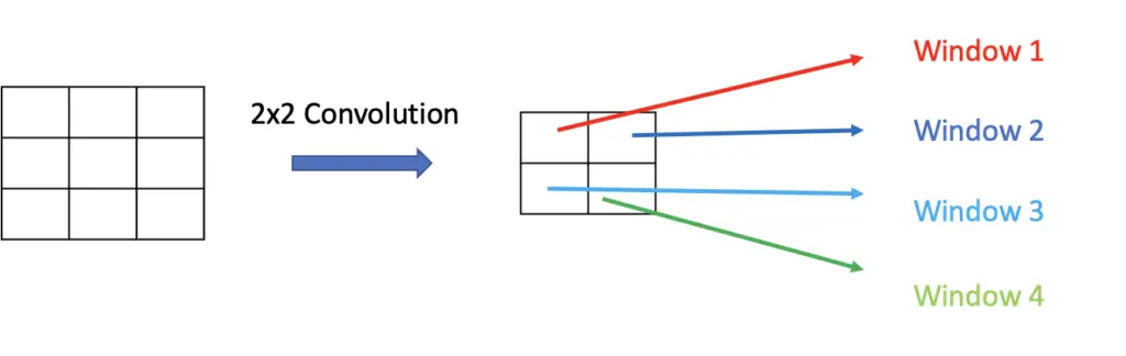
Convolutional neural networks are essentially image classification algorithms. You can turn a CNN into a model for object detection by finding regions in an image that potentially contain objects and use the neural network to classify whether the desired object is present in the image or not. The brute force approach would be a naive sliding window algorithm where you take windows of different sizes, slide them over the image, and have the neural network classify whether there is an object or not. Unfortunately, this approach isn’t very efficient since you have the network produce thousands of classifications on every single image.

To speed up the process of finding areas of the image that potentially contain objects of interest, the computer vision research community has come up with a set of region proposal algorithms. As the name implies, these algorithms identify regions in the image that potentially contain objects of interest. The network then only needs to adjust those regions and classify the objects contained inside of them.

Selective Search

The earlier object detection networks such as RCNN used an algorithm called selective search to identify areas of interest. In a nutshell, selective search is a graph-based clustering algorithm that groups regions of interest on the basis of features such as color, shape, and texture. A selective search algorithm will propose a couple of thousand regions.

Region Proposal Network

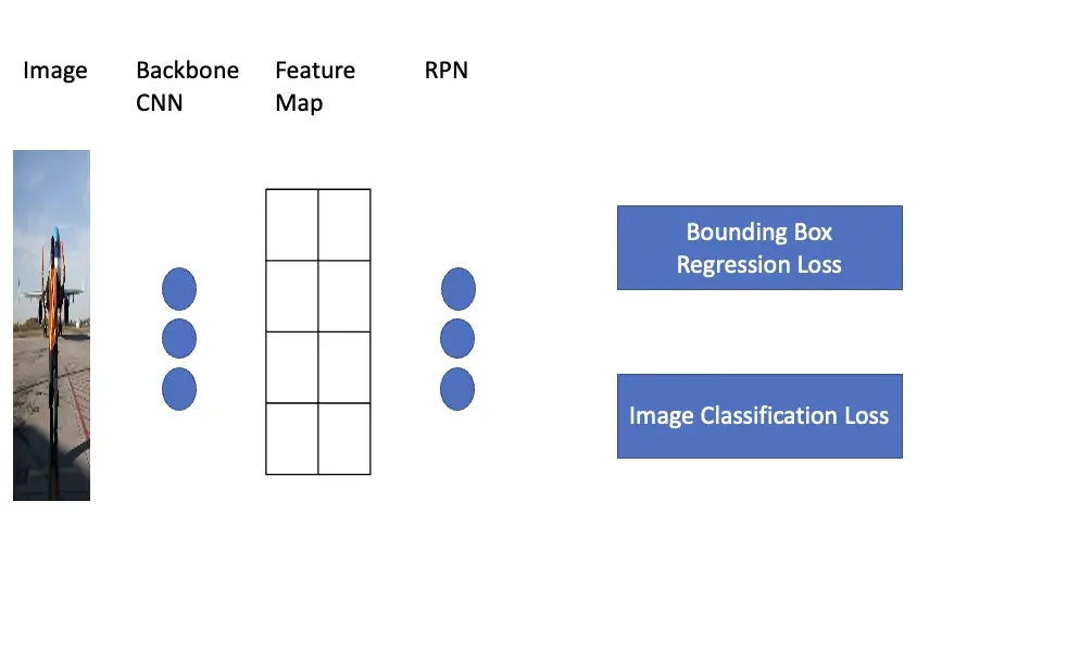
A region proposal network is a faster way to find areas of interest in an image and has been used in newer object detection networks such as Faster-RCNN. The basic idea of region proposal networks is to run your image through the first few layers of a convolutional neural network for object classification. A CNN for classification produces a series of shrinking feature maps through convolutional layers and pooling layers. It usually ends with fully connected layers that produce a classification. In a regional proposal network, you exclude the fully connected layers and use the feature map directly. Since the feature map will be much smaller than the original image, you can perform bounding box regression and object classification on much fewer windows.

The region proposal network is essentially a convolutional implementation of the sliding windows approach. For a more detailed explanation of the convolutional sliding windows approach, check out my post on the foundations of deep learning for object detection.

Region-Based Convolutional Neural Network (RCNN)

The region-based convolutional neural network was one of the first networks that successfully applied deep learning to the problem of object detection.

It works by initially applying the selective search algorithm to find region proposals. The proposals are then extracted and warped to a standard size so they can be processed by a neural network. Next, you apply a standard convolutional neural network to classify the images into one of several classes.

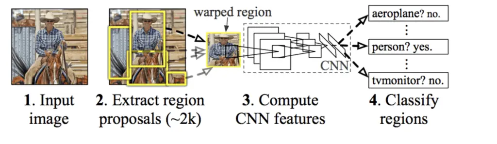
If we stopped there, we would potentially face the issue that the bounding boxes produced by selective search don’t match up with the objects we want to detect. The CNN is trained to classify specific objects, but the selective search algorithm doesn’t know which objects these are. To correct the region proposals from selective search, we also train the convolutional neural network to perform bounding box regression.

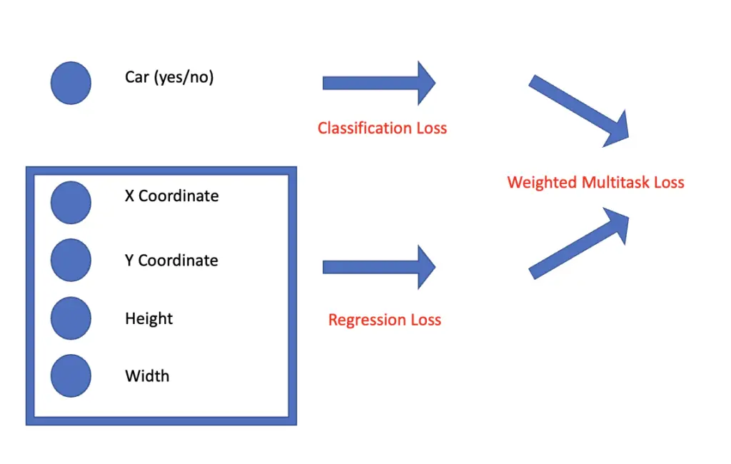
This means that the network performs a classification to detect whether an object of interest is present or not. In addition, it produces a transform to adjust the bounding boxes produced by the region proposal algorithm.

The regions proposal algorithm produces the x and y coordinates of the bounding box midpoint as well as the height h and width w of the box. The bounding box transform produced by the neural network is a set of 4 numbers {tx, ty, tw, th} that are multiplied with the original height and width values and added to the original coordinates to produce a translation of the original bounding box in the image coordinate system.

x_{new} = x + wt_x \;\;\;\; y_{new} = y +ht_y

The original height and width produced by the region proposal algorithm are scaled by multiplying them with the exponentiated value of the transform produced by the network.

w_{new} = w \times exp(t_w) \;\;\;\; h_{new} = h \times exp(t_h)

Since these are continuous numeric outputs, the network performs a regression. The regression part and the classification part require different loss functions that are subsequently combined in a weighted multitask loss.

Based on the multitask loss, you can train your neural network to produce the classifications and bounding-box transforms. As the last step, you need to filter through the boxes. Remember, the original region proposal algorithm produced thousands of images. There are several methods available for selecting the best bounding boxes. For a discussion of those methods, refer to my post on the foundations of deep learning for object detection.

Fast RCNN

A major drawback of RCNN is that it is extremely slow. After all, you have thousands of sub-images corresponding to region proposals, and you have to send them through the neural network individually. Extracting all the regions and sending them through the network for classification took tens of seconds per image. For real-time applications such as self-driving cars, this delay is unacceptable.
Furthermore, no learning is happening on the part of the region proposal algorithm since RCNN was using selective search, not a neural network.

Fast RCNN addressed these issues by running the image through a convolutional neural network before performing classification on the subregions. As discussed above, this network, known as the backbone network, extracts a feature map using a convolutional approach. Then you use a region proposal method such as selective search to find regions of interest in the feature map and use a convolutional neural network to classify those subregions. Instead of ending up with thousands of sub-images that have to be classified individually, you have very small features in the feature map. Classifying those features individually is much faster than classifying the sub-images produced by selective search. Due to the conventional operation performed before, we have a large degree of feature overlap/sharing between the features on the map. Bounding boxes are proposed on the basis of the spatial location of the feature inside the feature map.

Faster RCNN

While performing region proposals on a single feature map helped speed up Fast RCNN significantly, it still relied on selective search to find regions of interest. Faster RCNN managed to improve speed even further by using a region proposal network instead of applying selective search.

YOLO

You only look once (YOLO) marks a break with the previous approach of repurposing object classification networks for object detection. Yolo breaks new ground by using a single fully connected layer to predict the locations of objects in an image, essentially requiring only a single iteration to find the objects of interest. This results in a massive acceleration at inference time compared to previous architectures like RNN.

The fully connected layer that produces the location of the objects of interest has the following dimensions:

number\;of \;grids \,\times\; anchor\;boxes\;\times\;( \;class\; +bounding\;box\;coordinates\;+\;num\;classes)

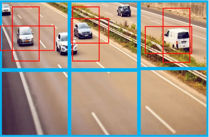
In the example above, we split the image into a 2 x 3 grid. We use two types of anchor boxes (one that is very high but not very wide, and another one that is wide but not very high). Then we have another neuron in the fully connected layer that expresses the confidence that the class is pr sent or not. The bounding box has 4 values (the width and height, as well as the x and y coordinates of its center). Lastly, we also have one neuron for every class that we are tryi g to detect. Since we only detect one class, we could theoretically do away with it, but let’s keep it for completeness’ sake.

Accordingly, you end up with the following dimensions.

2 \times 3 \times 2 \times ( 1 + 4 + 1)

The YOLO architecture looks very much like an image classification architecture. It has several convolutional and pooling layers that extract features from the image followed by two fully connected layers in the end they generate the final predictions.

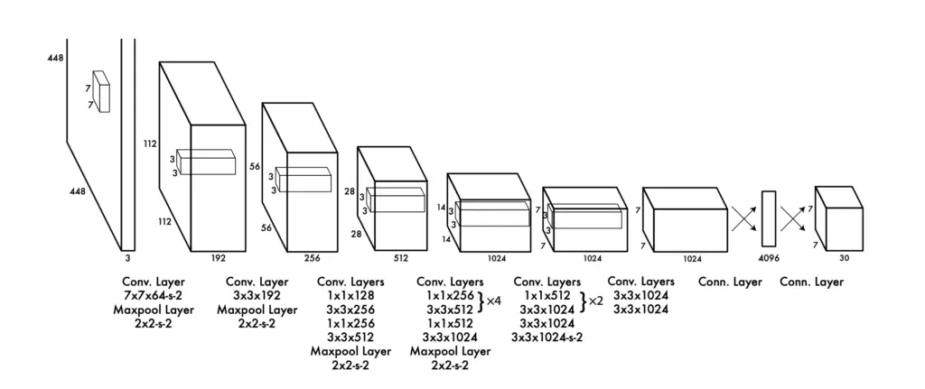
The convolutional layers extract the grid cells and the fully connected layers then output the confidence scores that the object of interest is present. In practice, you end up with a probability map where each section of one or several grid cells of the image is associated with a probability that a certain object is present.

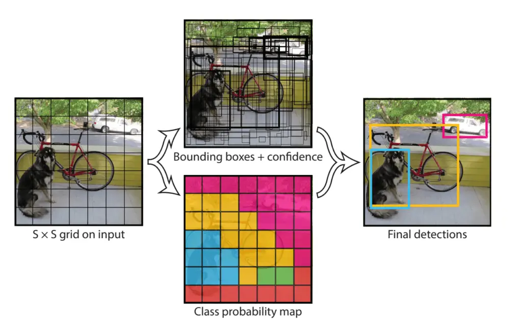
Of course, your network will produce a lot of bounding boxes initially. You get rid of them at training time by calculating the intersection over union with the ground-truth bounding box. At test time, you narrow down your choice of boxes by eliminating those associated with a low probability. Ultimately, you use non-max suppression to generate the final bounding-box predictions.

THe speed advantage of YOLO comes from its ability to run the whole image through the network once, split the image into grid cells, and predict whether a object is present or not. An disadvantage of this approach is that each grid cell can only predict one class. Accordingly, it loses accuracy when you have to deal with multiple tiny objects in the same location.

SSD

To correct the shortcomings of YOLO, computer vision researchers presented SSD in 2015. Like YOLO, SSD relies on a convolutional backbone network to extract feature maps. But it doesn’t rely on 2 fully connected layers to produce the bounding boxes. Instead, it stacks several convolutional layers that produce progressively smaller feature maps. At each size, the network produces a score for each grid cell to determine how well the cell matches the desired object. This allows SSD networks to scale the bounding box to the size of the desired object and thus detect objects of different sizes. Compared to YOLO, SSD is more accurate because of its ability to produce bounding boxes at different scales. Of course, it also produces a much larger number of bounding boxes resulting in slight losses in speed compared to YOLO. Nevertheless, SSD is still orders of magnitude faster than the original RCNN architectures.

Conclusion

The RCNN family constituted the first neural network architectures in the deep learning era for object detection. RCNNs combined traditional, graph based algorithms for region proposal with neural networks for object classification. While they delivered good results, the first generations were extremely slow.
Further RCNN iterations significantly improved detection speed by introducing neural networks and convolutional operations to handle region proposals.

YOLO significantly improved detection speed by passing input through a neural network only once. It relied on fully connected layers to produce both object classifications, as well as the locations of the bounding boxes.

SSD corrected some of the shortcomings of YOLO by producing bounding boxes at different scales.

This article is part of a blog post series on deep learning for computer vision. For the full series, go to the index.