How to Perform Matrix Multiplication
In this post we learn how to perform matrix multiplication and why we need to be mindful of matrix dimensions. Furthermore, we look at the properties of matrix multiplication.
Matrix multiplication is an operation that consists of the element-wise multiplication of all entries in a row of the first matrix with all entries in the column at the same index as the row of the first matrix followed by the summation of all products. The result is a new matrix. This process is more commonly known as the dot product and can be applied to matrices and vectors alike.
Matrix multiplication is perhaps the most important matrix operation. There are different forms of matrix multiplication, but the row-column-wise dot product described above is the most common one. In areas like machine learning, matrix multiplication is central to many algorithms such as neural networks,
Matrix Vector Multiplication
Matrices can be multiplied with a vector by taking the dot product of each row of an m \times n matrix A with the n-dimensional vector b. You can imagine the matrix A as several vectors {a_1, a_2, …, a_m } stacked on top of each other.
Since you are multiplying matrix rows with vector columns, an important precondition is that A has the same number of columns as the vector has rows.
So if you have an m \times n matrix A, the vector b needs to have n entries. The product will be an m \times 1 vector c.
c =
   \begin{bmatrix}
    a_{11} & ... & a_{1n}  \\
    ... & ... & ... \\
    a_{m1} & ... & a_{mn}  \\

  \end{bmatrix}
\begin{bmatrix}b_1\\...\\b_n\end{bmatrix}
=
\begin{bmatrix}c_1\\...\\c_m\end{bmatrix}
For example:
 c =
 \begin{bmatrix}
    3 & 2 \\
    4 & 3 \\
    4 & 3 \\

  \end{bmatrix}


\times

  \begin{bmatrix}
    2 \\
    3 \\

  \end{bmatrix}
=
  \begin{bmatrix}
    12 \\
    17  \\
    17 \\

  \end{bmatrix}
Matrix Matrix Multiplication
Matrix multiplication or the dot product of matrices is very similar to matrix-vector multiplication. To perform matrix-matrix multiplication, you have to take the dot product of every row in m \times n matrix A with every column in n \times k matrix B.
Imagine A as several vectors { a_1, a_2, …, a_m} stacked horizontally on top of each other and B as several vectors {b_1, b_2, …, b_k } stacked vertically next to each other.
As with matrix-vector multiplication, A needs to have the same number of columns as B has rows.
  C=
 \begin{bmatrix}
    a_{11} & ... & a_{1n}  \\
    ... & ... & ... \\
    a_{m1} & ... & a_{mn}  \\

  \end{bmatrix}
   \begin{bmatrix}
    b_{11} & ... & b_{1k}  \\
    ... & ... & ... \\
    b_{n1} & ... & b_{nk}  \\

  \end{bmatrix}
=
   \begin{bmatrix}
    c_{11} & ... & c_{1k}  \\
    ... & ... & ... \\
    c_{m1} & ... & c_{mk}  \\

  \end{bmatrix}
For example:
C=
  \begin{bmatrix}
    3 & 2 \\
    4 & 3 \\
    4 & 3 \\

  \end{bmatrix}


\times

  \begin{bmatrix}
    1 & 1 & 1 & 1 \\
    2 & 2 & 2 & 2 \\

  \end{bmatrix}
=
  \begin{bmatrix}
    7 & 7 & 7 & 7 \\
    10 & 10 & 10 & 10 \\
    10 & 10 & 10 & 10 \\


  \end{bmatrix}
where
c11 = 3 x 1 + 2 x 2 = 7 c12 = 3 x 1 + 2 x 2 = 7 …
c21 = 4 x 1 + 3 x 2 = 10 c22 = 4 x 1 + 3 x 2 = 10 …
This process can be neatly summarised using Einstein-summation. An entry in C c_{mk} can be calculated as follows:
c_{mk} = \sum\limits_{n=1}^N a_{mn}b_{nk}Matrix Dimensions
If you have an m \times n matrix A, and an n \times k matrix B, the product will be a n \times k matrix, since you are taking the dot product of each row in A with each column in B.
What I like to do is write the dimensions down like this:
(m \times n) (n\times k) = (m\times k) \\ A\,\,\,\,\,\,\,\,\,\,\,\,\,\,B\,\,\,\,\,=\,\,\,\,\,\,\,\,C
So the two inner terms (n) have to match, while the two outer terms m and k define the dimensions of the new matrix C
Examples
To solidify your understanding, here are some more examples for 2×2 and 3×3 matrices.
2×2 Matrix Multiplication
  \begin{bmatrix}
    1 & 2 \\
    3 & 4 \\
  \end{bmatrix}


\times

  \begin{bmatrix}
    2 & 2 \\
    3 & 3 \\

  \end{bmatrix}

=
  \begin{bmatrix}
    8 & 8 \\
    18 & 18 \\
  \end{bmatrix}
3×3 Matrix Multiplication
  \begin{bmatrix}
    3 & 2 & 2 \\
    4 & 3 & 4 \\
    4 & 3 & 5 \\

  \end{bmatrix}


\times

  \begin{bmatrix}
    3 & 2 & 2 \\
    4 & 3 & 4 \\
    4 & 3 & 5 \\

  \end{bmatrix}
=
  \begin{bmatrix}
    25 & 18 & 24 \\
    40 & 29 & 40 \\
    44 & 32 & 45 \\

  \end{bmatrix}
Matrix Multiplication Properties
Matrix multiplication has some properties that you should be aware of.
Is Matrix Multiplication Commutative?
Since we are multiplying the rows of the first matrix, with the columns of the second matrix, matrix multiplications are not commutative. If we changed the order of our elements we’d get a different product.
For example:
  \begin{bmatrix}
    1 & 2 \\
    3 & 4 \\
  \end{bmatrix}


\times

  \begin{bmatrix}
    2 & 2 \\
    3 & 3 \\

  \end{bmatrix}
=
  \begin{bmatrix}
    8 & 8 \\
    18 & 18 \\
  \end{bmatrix}
\begin{bmatrix}
2 & 2 \\
3 & 3 \\
\end{bmatrix}
\times
\begin{bmatrix}
1 & 2 \\
3 & 4 \\
\end{bmatrix}
=
\begin{bmatrix}
8 & 10 \\
12 & 18 \\
\end{bmatrix}
In most cases switching the order is impossible because the dimensions don’t match. If you took a 4×3 matrix A and a 3×2 matrix B, AxB is possible, but BxA is not.
Is Matrix Multiplication Associative?
Matrix multiplication is associative. In a multiplication involving three matrices A, B, C, it doesn’t matter whether you first multiply a matrix A with B or B with C, therefore
(AB)C=A(BC)
But as discussed, you cannot change the order of the matrices.
Is Matrix Multiplication Distributive?
Matrix multiplication is only partly distributive. The following properties hold for matrix multiplication
A(B+C)=AB+AC
(B+C)A=BA+CA
whereas A(B+C) \neq (B+C)A does not hold:
Summary
We’ve learned to multiply matrices and why we need to be mindful of matrix dimensions. We also discussed the properties of matrix multiplication
You now have an understanding of the foundational building blocks of linear algebra: vectors and matrices. The real power comes from combining them to transform and warp multidimensional spaces according to your needs.
This is a real superpower which can be applied to many disciplines. Regardless of whether you go into data science, machine learning, mechanical engineering, quantum physics or any other technical discipline.
This post is part of a series on linear algebra for machine learning. To read other posts in this series, go to the index.


