The Law of Total Probability and Bayesian Inference

In this post we introduce the law of total probability and learn how to use Bayes’ rule to incorporate prior probabilities into our calculation for the probability of an event.

Events don’t happen in a vacuum. They are related to and dependent on circumstances in their environment. Bayes rule allows us to relate the prior probability for an event arising from circumstances such as age risk for a disease, to the probability of the actual event happening.

Formally, Bayes theorem says that the probability that an event A happens given B is the probability of B happening given A multiplied by the marginal probability of A divided by the marginal probability of B.

P(A|B) = \frac{P(B|A)P(A)}{P(B)}

This gives rise to some very interesting statistical properties.

The Law of Total Probability

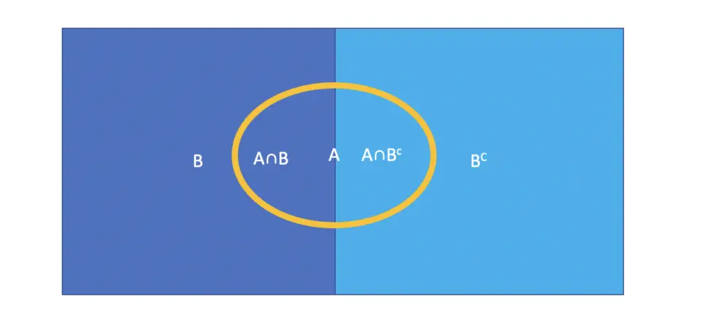
The law of total probability says that the probability of an Event A can be calculated as the sum of the intersections of A with the events B and its complement BC that fills up the sample space.

P(A) = P(A \cap B) + P(A \cap B^C)

Using chain rule of conditional probability we can express the law of total probability as follows.

P(A) = P(A|B)P(B) + P(A|B^C)P(B^C)

Example For Bayesian Inference and the Law of Total Probability

For example, if a person tests positive for lung cancer there is a chance that the result is a false positive and the person actually doesn’t have lung cancer. Let’s say the test is accurate 99% of the time in determining lung cancer. In statistics, this true positive rate is called the test sensitivity.

Does that mean the person is 99% likely to have lung cancer?

Luckily for the patient, the actual probability is much smaller.

Let’s assume the chance of developing lung cancer in any given year (the prior probability) is 0.07%. I’m going to ignore factors like age or smoking that affect your risk. Let’s also assume the chance of testing positive even though the person does not have cancer, is 3%. This is called the false positive rate.

Using Bayes’ rule, we can incorporate the prior probability to calculate the actual probability that the person has lung cancer given a positive test result.

P(Cancer|Positive) = \frac{P(Positive|Cancer)P(Cancer)}{P(Positive)}

Let’s first define our probabilities. The true positive rate is basically the probability that the person has a positive test result given that he has lung cancer.

P(Positive|Cancer) = 0.99

The general probability of getting cancer is 0.07%

P(Cancer) = 0.0007

Calculating P Positive

We still need P(Positive), the probability that a test is positive regardless of whether the person has lung cancer or not. Applying the law of total probability, we can calculate this as the probability that someone tests positive times the probability of getting cancer, plus the probability that someone without cancer tests positive times the probability of not having cancer

P(Positive) \\
= P(Positive|Cancer)P(Cancer)  \\
+ P(Positive|NoCancer)P(NoCancer) 

The probability of not having cancer is 1 minus the probability of having cancer.

P(NoCancer) = 1 - P(Cancer) = 1 - 0.0007 = 0.9993

The false positive rate is 0.03 as specified above.

P(Positive|NoCancer) = 0.03

Finally, we can calculate P(Positive)

P(Positive) = 0.99 \times 0.0007 + 0.03 \times 0.9993 = 0.03

Calculating the Posterior Probability

Now, we can plug this into Bayes’ theorem.

P(Cancer|Positive) = \frac{0.99 \times 0.0007}{0.03} = 0.023

In other words, the chance of having lung cancer given a positive test is actually only 2.3%.

For people who have never encountered Bayesian statistics, this might sound shocking. Does this mean the test is nonsense? No, it doesn’t! Relatively speaking, your probability of having lung cancer has increased 33-fold from 0.07% to 2.3%.

But in this case, the prior odds of not having cancer are so strongly in your favor, that even a highly accurate test will not give you a high absolute probability.

Summary

We’ve learned how to incorporate prior probabilities into our calculation for the probability that an event occurs using Bayes’ rule.

You’ve seen that the prior probability can have a huge impact on the posterior outcome. The probability of having a disease can go from almost certainty to unlikely. This effect is strongest in scenarios that are highly unlikely to begin such as developing a rare disease.

I hope this also gives you a sense of why so many predictions are wrong. In many cases, the probability of a prediction coming true is highly contingent on the prior probability. But when the environment is dynamic and complex like modern financial markets, it is next to impossible to correctly assess the correct prior probability. For the sake of your own financial wellbeing, never trust anyone who tells you that markets will crash next month. It is impossible that that person has correctly assessed all the prior probabilities. If he or she happens to be right, it is pure coincidence. You might as well let a dart-throwing chimp make that prediction for you.

This post is part of a series on statistics for machine learning and data science. To read other posts in this series, go to the index.