Building a Neural Network with Training Pipeline in TensorFlow and Python for the Titanic Dataset: A Step-by-Step Example

In this post, we will cover how to build a simple neural network in Tensorflow for a spreadsheet dataset. In addition to constructing a model, we will build a complete preprocessing and training pipeline in Tensorflow that will take the original dataset as an input and automatically transform it into the format necessary for model training.
Getting Set Up
Note: If you already have a jupyter notebook with Tensorflow and Python up and running, you can skip to the next section.
Before we can build a model in TensorFlow, we need to set up our machine with Python and Tensorflow. I assume that you already have Python installed along with a package manager such as pip or conda. If that isn’t the case, you need to do that before you can continue with this tutorial. Here is a great tutorial on installing Python.
Navigate to the directory where you want to work and download the Titanic Dataset from Kaggle to your working directory. Unzip the package. Inside you’ll find three CSV files.
It is generally good practice to set up a new virtual Python environment and install Tensorflow and your other dependencies into that environment. That way, you can manage different projects that require different versions of your dependencies on the same machine. Furthermore, it is much easier to export the required dependencies.
I am using conda for managing my packages. Open a terminal window (I’m on macOS, on Windows, use an alternative like Putty) and navigate to your working directory.
cd path/to/your/working/directory
Next, I am telling conda to create an environment with Python 3.8.
conda create --name titanic python=3.8
conda activate titanic
Now we need to install our dependencies. Besides Tensorflow, we install some basic Python packages for data manipulation as well as jupyter to run Jupyter notebooks. The standard pip installation of Tensorflow will give you the latest stable version with both GPU and CPU support. For this tutorial, we won’t need GPU support, but once you are running larger workloads, I highly recommend it.
pip install jupyter pandas matplotlib scikit-learn, seaborn
pip install tensorflow
I ran into an error while importing NumPy with the standard pip installation. At the time of this writing, the latest NumPy package seems incompatible with Python 3.8, so I did another pip install specifying an earlier version.
pip install numpy==1.21.5
Start the jupyter notebook server by typing the following command into your terminal.
jupyter notebook
Importing the Data and Performing an Initial Analysis
Create a new jupyter notebook, open it, and import the libraries we’ve installed in the previous section.
import numpy as np
import pandas as pd
import seaborn as sns
import tensorflow as tf
We will just import the train.csv file as a pandas data frame from the titanic data directory that we’ve downloaded before.
data= pd.read_csv('titanic/train.csv')
We first look at the data to understand its shape.
print(data.shape)
data.head()
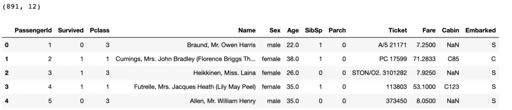
This is a record of 891 people who traveled on the Titanic when it sank. We want to predict who survived based on the remaining features in the dataset.
Let’s plot the variable “Survived” to see how it is distributed (how many people perished and how many survived).
sns.countplot(data=data,x='Survived')
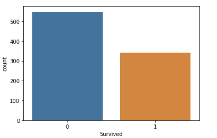
It seems like more than 500 people died, and somewhat over 300 survived. It is important to keep in mind that the classes are not balanced because the model could achieve well over 60% accuracy by simply predicting that everyone died.
Next, we will use our own intuition to filter the data and select the relevant features. When looking at the data, I’ve guessed that class, fare, age, and sex are probably important predictors. People who traveled in the first class and paid a higher fare were given priority over people in the lower classes. Women and children were probably also more likely to be saved. Of course, this is just my intuition.
If your goal is to find the best model possible, you wouldn’t just rely on your intuition but do more preliminary analysis, tinker around with the data and investigate if there are correlations between survival and other features.
But our goal here is to build a neural network and an input pipeline that automates the whole process. For this tutorial, we don’t care about achieving the highest possible accuracy.
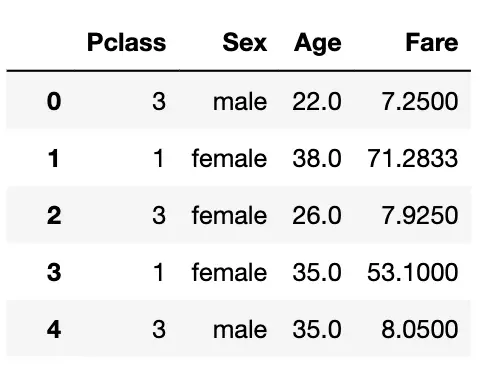
I’m going to filter the data for the selected variables.
data = data[['Survived', 'Pclass', 'Sex', 'Age', 'Fare']]
Next, we want to get rid of all null values in the data. Pandas makes this easy.
data = data.dropna()
print(data.shape) #(714, 4)
If you want to achieve the highest possible accuracy, you might not want to simply drop the values that contain a null entry since you are throwing away a lot of useful information in the other features.
Before we can start building the input pipeline, we want to separate the predicted variable from the predictors.
target = data.pop('Survived')
Building the Machine Learning Pipeline in TensorFlow
A large part of any machine learning project is spent on data manipulation and preprocessing before the data is suitable for training. If you want to deploy a model into production, you need to automate the process of preprocessing and transforming the data into a format suitable for model training.
What Data Format is Required for Training a Neural Network?
If we look at the remaining predictors, we see that Pclass is a categorical feature expressed in integer values. There are a total of three classes, and a passenger falls into one of them. Sex is another categorical variable because passengers are either classified as male or female, and the classification is expressed in strings. The age and fare columns contain continuous numeric values.
Before we feed the values to a neural network, we should normalize the numeric values, and one-hot encode the categorical variables.
Normalization ensures that all numeric features are on a similar scale from 0 to 1, which helps speed up gradient descent. If you are unclear why normalization helps gradient descent, check out my post on data normalization.
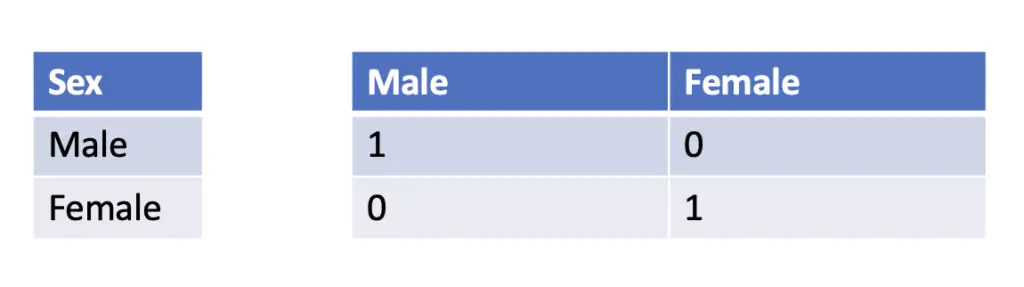
One hot encoding creates a new column for every category in a variable. It then fills all row entries of each column with zeros except for the rows that actually contain that category.
For example, if. one row in the original column contained the entry “male”, and the second contained “female”, we would end up with two columns named “male”, and “female” with 1s in the row that contained the original category.
This may look like an unnecessary complication. We one-hot encode data because neural networks need numeric data to learn. But why can’t we just map every string category to a corresponding integer? It is possible in cases where a natural ordering exists in the data. But the network may infer an order that doesn’t exist in this case. For example, we don’t want the network to conclude that males are preferable to females. Giving every category its own column essentially binarizes the problem, which removes the potential for implicit ordering.
The survival status, our predicted variable, is another categorical feature expressed in integer values. If the person has survived, it is indicated by the value 1. Death is indicated by a 0. To be precise, survival is a binary feature, and since it only contains 0s and 1s, we don’t need to apply any transformation.
So we split our feature columns between categorical features, numeric features, and the predicted variable.
categorical_feature_names = ['Pclass','Sex']
numeric_feature_names = ['Fare', 'Age']
predicted_feature_name = ['Survived']
Convert the Dataframe to Tensors
To feed the data frame to TensorFlow specific functions, we need to process it into a data object that Tensorflow can work with. To achieve this, we define a Keras tensor for every column in our dataset that acts as a placeholder for the actual data we pass at runtime.
In the following function we:
- iterate through the columns,
- identify the datatype of the column and assign a corresponding tensorflow datatype,
- create the tensor with the datatype and a yet undefined shape,
- pull the tensors into a dictionary and uniquely identify each by the name of the column.
def create_tensor_dict(data, categorical_feature_names):
inputs = {}
for name, column in data.items():
if type(column[0]) == str:
dtype = tf.string
elif (name in categorical_feature_names):
dtype = tf.int64
else:
dtype = tf.float32
inputs[name] = tf.keras.Input(shape=(), name=name, dtype=dtype)
return inputs
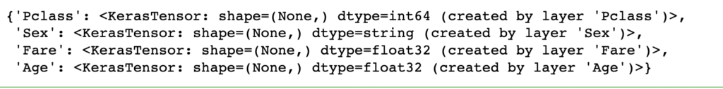
inputs = create_tensor_dict(data, categorical_feature_names)
print(inputs)
Normalize the Input in TensorFlow
Before we normalize the numeric features, we define a helper function that converts the numeric columns from our pandas’ data frame into tensors of floats and stacks them together into one large tensor.
def stack_dict(inputs, fun=tf.stack):
    values = []
    for key in sorted(inputs.keys()):
      values.append(tf.cast(inputs[key], tf.float32))

    return fun(values, axis=-1)
Next, we create the normalizer. We first filter the numeric feature columns from the dataframe. Then we instantiate Keras’ inbuilt normalizer, tell it to normalize along the last axis of our tensor, and adapt the normalizer to our features which we’ve converted to a dictionary, and then to a tensor using the helper function.
def create_normalizer(numeric_feature_names, data):
    numeric_features = data[numeric_feature_names]

    normalizer = tf.keras.layers.Normalization(axis=-1)
    normalizer.adapt(stack_dict(dict(numeric_features)))
    return normalizer
Finally, we perform the actual normalization in a new function to which we pass the normalizer. In the previous function, we’ve told the normalizer to expect a stacked dictionary of tensors. Previously, we’ve defined a dictionary that contains placeholder tensors for the model. At runtime, the model will expect an input of that same format. Therefore, we need to bring the dictionary into a format that our normalizer can process.
If we filter the dictionary down to just the placeholders for the numeric features and stack them using the stackdict function, we can pass them to the normalizer.
def normalize_numeric_input(numeric_feature_names, inputs, normalizer):
    numeric_inputs = {}
    for name in numeric_feature_names:
      numeric_inputs[name]=inputs[name]

    numeric_inputs = stack_dict(numeric_inputs)
    numeric_normalized = normalizer(numeric_inputs)
    return numeric_normalized
Now we can create the normalizer and subsequently normalize the data using the two functions. This will result in a tensor in which the numeric features have been stacked along the y-axis. Since our data has two numeric feature columns, the y-axis will have 2 entries.
normalizer = create_normalizer(numeric_feature_names, data)
numeric_normalized = normalize_numeric_input(numeric_feature_names, inputs, normalizer)
print(numeric_normalized)

Ultimately, we want to collect all preprocessed features together so that we can feed them to the model as one dataset. We start by creating an empty list of preprocessed features, to which we gradually add the features as we process them.
preprocessed = []
preprocessed.append(numeric_normalized)
One Hot Encode Categorical Features in TensorFlow
We’ve processed the numerical features. As a next step, we want to one-hot encode the categorical features. Remember that we have categorical features that are encoded either as strings or as integers. Specifically, we need to distinguish between 3 classes and 2 sexes.
In the following function, we iterate through the columns in our dataframe that contain categorical features. We then check if the data contained is of type string or of type integer. In the first case, we define a lookup function to convert the column into a one-hot encoding on the basis of the contained string values. In the second case, we define an integer lookup function to achieve the same thing.
We then retrieve the placeholder from the inputs dictionary corresponding to the column, apply the previously defined lookup function to it, and retrieve the resulting one-hot encoding of the column.
Ultimately, we collect all one hot encodings in a list that we return from the function.
def one_hot_encode_categorical_features(categorical_feature_names, data, inputs):
    one_hot = []
    for name in categorical_feature_names:
      value = sorted(set(data[name]))

      if type(value[0]) is str:
        lookup = tf.keras.layers.StringLookup(vocabulary=value, output_mode='one_hot')
      else:
        lookup = tf.keras.layers.IntegerLookup(vocabulary=value, output_mode='one_hot')

      x = inputs[name][:, tf.newaxis]
      x = lookup(x)
      one_hot.append(x)
    return one_hot
The result is a list of tensors of categorical one-hot encoded features. We can, therefore directly add it to the list of preprocessed tensors.
one_hot = one_hot_encode_categorical_features(categorical_feature_names, data, inputs)
preprocessed = preprocessed + one_hot
print(preprocessed)

We now have a list of 3 tensors. But we want to feed one large tensor to the model, which is why we concatenate the results along the y-axis.
preprocesssed_result = tf.concat(preprocessed, axis=-1)
print(preprocesssed_result)

Tensorflow automatically numbers the layers. Depending on how often you have executed the functions, you will see different numbers in the layer names.
Building the Model
We are now in a position to build a model that automates the preprocessing on the basis of the functions we’ve defined before.
Define the Preprocessing Layer
To instruct Keras to perform the preprocessing, we construct a new model. Then we have to pass the input in the expected format (the dictionary of tensor placeholders defined in the beginning) and the output in the expected format. The model now automatically applies all the intermediate functions defined before that are necessary to go from the input to the expected output.
preprocessor = tf.keras.Model(inputs, preprocesssed_result)
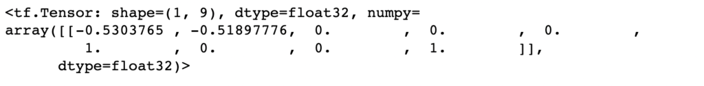
To test that the preprocessor works, we pass it the first row of our dataset converted to a dictionary. That way, it should have the expected format as expressed by the placeholder input dictionary. We should get a 1×9 dimensional tensor (1 because we only passed it one row and 9 because we have a total of 9 columns).
preprocessor(dict(data.iloc[:1]))
Build the Neural Network
We use Keras’ sequential API to define the neural network. Since the use case is spreadsheet data, a simple feedforward multilayer perception should be enough. We use two dense hidden layers with 10 neurons each and apply the conventional ReLU activation function. In the output layer, we use the sigmoid activation function since we have a binary classification problem.
network = tf.keras.Sequential([
  tf.keras.layers.Dense(10, activation='relu'),
  tf.keras.layers.Dense(10, activation='relu'),
  tf.keras.layers.Dense(1)
])
Next, we tie the preprocessor and the network together into one model.
x = preprocessor(inputs)
result = network(x)
model = tf.keras.Model(inputs, result)
Take note of the brilliant simplicity of the Keras Functional API: The network and the preprocessor can each be defined as separate models. We can simply link them together into one unified model by passing the output from the preprocessor as an input to the network.
Finally, we compile the model using the Adam optimizer (we could also use another one, but Adam is generally a good default), binary cross-entropy as the loss function (because we have a binary optimization problem), and accuracy as the evaluation metric.
model.compile(optimizer='adam',
                loss=tf.keras.losses.BinaryCrossentropy(from_logits=True),
                metrics=['accuracy'])
We finally convert the data to a dictionary, so it has the expected format expressed by the placeholder dictionary and fit the model. Feel free to use a different batch size and number of epochs.
history = model.fit(dict(data), target, epochs=20, batch_size=8)
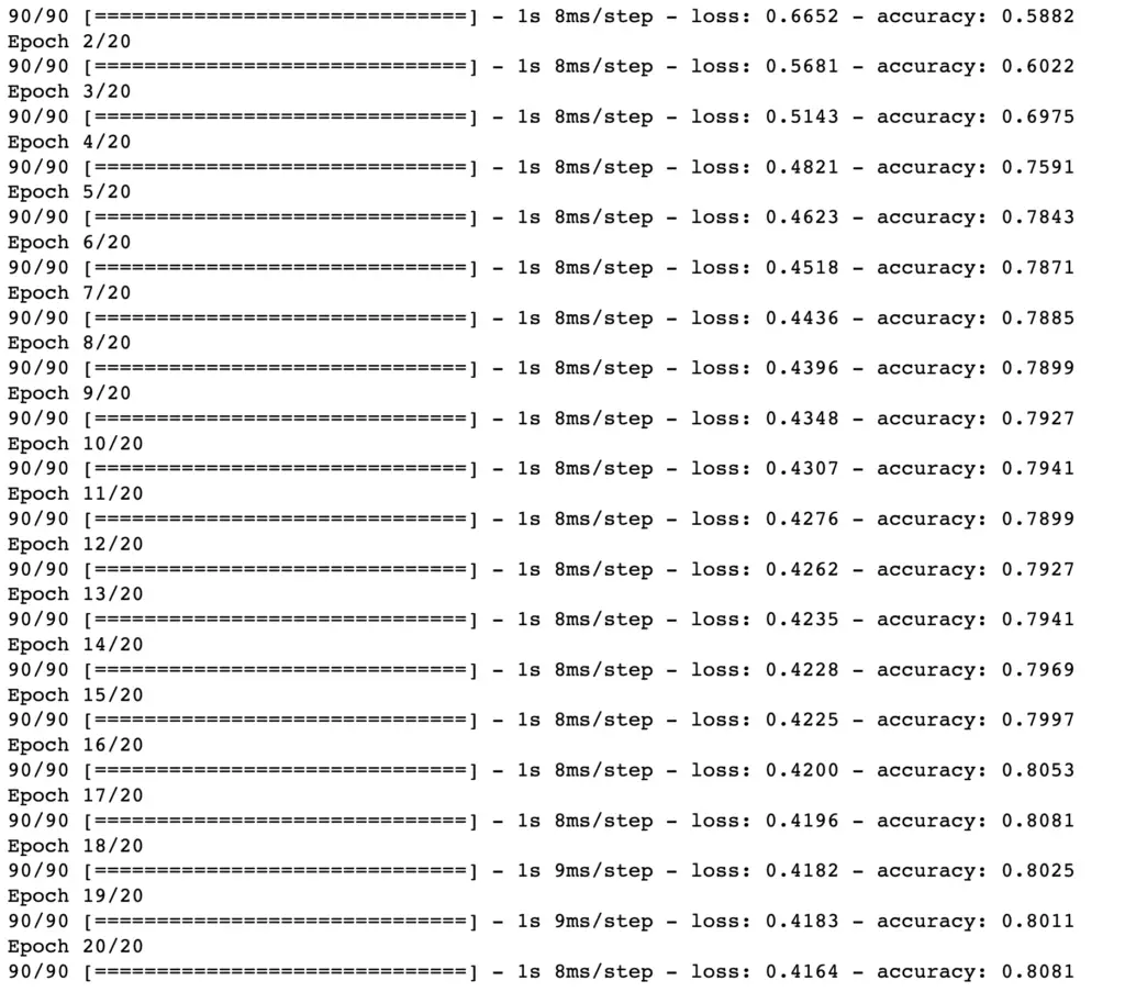
We’ve achieved an accuracy of 80%, which isn’t so bad. We could probably nudge that up a little bit by some more sophisticated feature engineering and playing with the model architecture.
Split the Data into Training and Validation Sets
You may have realized that we only trained the model on the training set. In the following function, we split the data between train and test based on a specified proportion. We chose an 80/20 split and fit the model.
def create_train_val_split(data, split):
    msk = np.random.rand(len(data)) < split
    train_data = data[msk]
    val_data = data[~msk]
    train_target = target[msk]
    val_target = target[~msk]
    return (train_data, val_data, train_target, val_target)


(train_data, val_data, train_target, val_target) = create_train_test_split(data, 0.8)
history = model.fit(dict(train_data), train_target, validation_data=(dict(val_data), val_target), epochs=20, batch_size=8)
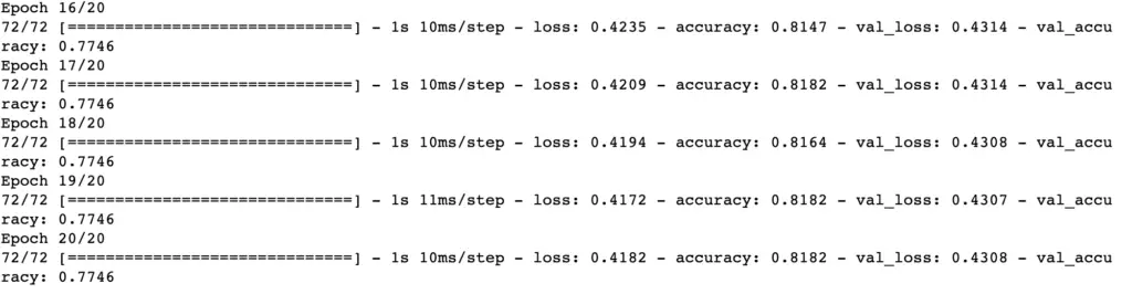
The validation accuracy is a few percentage points below the training accuracy. This dataset is fairly small, which is why you should expect some fluctuation in the results when you randomly split the data.
Instead of passing data and outcome separately, you can also pull them together into a TensorFlow dataset. This has the advantage that your model fit function is much more concise as you can specify the batch size and shuffle the data directly on the TensorFlow dataset before you call model fit.
#Alternatively
train_ds = tf.data.Dataset.from_tensor_slices((
    dict(train_data),
    train_target
))

test_ds = tf.data.Dataset.from_tensor_slices((
    dict(test_data),
    test_target
))

train_ds = train_ds.batch(8)
test_ds = test_ds.batch(8)

history = model.fit(train_ds, validation_data=test_ds, epochs=20)
Putting It All Together
As part of process automation, we also summarize the data manipulation we’ve performed in disparate steps during the initial analysis in a function. We essentially select the columns on the basis of the selected feature names, remove the columns containing null, and split the predicted variable from the predictors. The following functions are those that we have already defined before.
def preprocess_dataframe(data, categorical_feature_names, numeric_feature_names, predicted_feature_name):
    all_features_names = categorical_feature_names + numeric_feature_names + predicted_feature_name
    data = data[all_features_names]
    data = data.dropna()
    target = data.pop(predicted_feature_name[0])
    return (data, target)


def create_tensor_dict(data, categorical_feature_names):
    inputs = {}
    for name, column in data.items():
      if type(column[0]) == str:
        dtype = tf.string
      elif (name in categorical_feature_names):
        dtype = tf.int64
      else:
        dtype = tf.float32

      inputs[name] = tf.keras.Input(shape=(), name=name, dtype=dtype)
    return inputs


def stack_dict(inputs, fun=tf.stack):
    values = []
    for key in sorted(inputs.keys()):
      values.append(tf.cast(inputs[key], tf.float32))

    return fun(values, axis=-1)


def create_normalizer(numeric_feature_names, data):
    numeric_features = data[numeric_feature_names]

    normalizer = tf.keras.layers.Normalization(axis=-1)
    normalizer.adapt(stack_dict(dict(numeric_features)))
    return normalizer

def normalize_numeric_input(numeric_feature_names, inputs, normalizer):
    numeric_inputs = {}
    for name in numeric_feature_names:
      numeric_inputs[name]=inputs[name]

    numeric_inputs = stack_dict(numeric_inputs)
    numeric_normalized = normalizer(numeric_inputs)
    return numeric_normalized


def one_hot_encode_categorical_features(categorical_feature_names, data, inputs):
    one_hot = []
    for name in categorical_feature_names:
      value = sorted(set(data[name]))

      if type(value[0]) is str:
        lookup = tf.keras.layers.StringLookup(vocabulary=value, output_mode='one_hot')
      else:
        lookup = tf.keras.layers.IntegerLookup(vocabulary=value, output_mode='one_hot')

      x = inputs[name][:, tf.newaxis]
      x = lookup(x)
      one_hot.append(x)
    return one_hot


def create_train_val_split(data, split):
    msk = np.random.rand(len(data)) < split
    train_data = data[msk]
    val_data = data[~msk]
    train_target = target[msk]
    val_target = target[~msk]
    return (train_data, val_data, train_target, val_target)
Using these functions, we can load our data and build our training pipeline that ends with the neural network.
#Load data and specify desired columns
data= pd.read_csv('titanic/train.csv')
categorical_feature_names = ['Pclass','Sex']
numeric_feature_names = ['Fare', 'Age']
predicted_feature_name = ['Survived']

#Preprocess dataframe
(data, target) = preprocess_dataframe(data, categorical_feature_names, numeric_feature_names, predicted_feature_name)


#Create tensorflow preprocessing head
inputs = create_tensor_dict(data, categorical_feature_names)
preprocessed = []
normalizer = create_normalizer(numeric_feature_names, data)
numeric_normalized = normalize_numeric_input(numeric_feature_names, inputs, normalizer)

preprocessed.append(numeric_normalized)
one_hot = one_hot_encode_categorical_features(categorical_feature_names, data, inputs)
preprocessed = preprocessed + one_hot
preprocesssed_result = tf.concat(preprocessed, axis=-1)
preprocesssed_result

preprocessor = tf.keras.Model(inputs, preprocesssed_result)


#Define the model
network = tf.keras.Sequential([
  tf.keras.layers.Dense(10, activation='relu'),
  tf.keras.layers.Dense(10, activation='relu'),
  tf.keras.layers.Dense(1)
])
x = preprocessor(inputs)
result = network(x)
#result
model = tf.keras.Model(inputs, result)


model.compile(optimizer='adam',
                loss=tf.keras.losses.BinaryCrossentropy(from_logits=True),
                metrics=['accuracy'])
Now we can split the data frame into training and test set and directly fit the model on the data.
(train_data, val_data, train_target, val_target) = create_train_test_split(data, 0.8)
history = model.fit(dict(train_data), train_target, validation_data=(dict(val_data), val_target), epochs=20, batch_size=8)
Further Resources
For building the preprocessing head, I relied heavily on the official TensorFlow documentation on importing pandas dataframes into TensorFlow.
https://www.tensorflow.org/tutorials/load_data/pandas_dataframe#build_the_preprocessing_headThis article is part of a blog post series on the foundations of deep learning. For the full series, go to the index.
